Electromagnetism Resource
| Site: | WelTec Moodle |
| Course: | New Zealand Certificate in Electrical Engineering Theory (Level 3) Stream B (2020) |
| Book: | Electromagnetism Resource |
| Printed by: | Guest user |
| Date: | Saturday, 2 May 2026, 7:12 AM |
Description
Table of contents
- 1. Introduction
- 2. Vectors and Vector Fields
- 3. Electric and Magnetic Fields
- 4. Electromagnetic Effects
- 4.1. Magnetic Fields of Single Wires and Coils
- 4.2. Force Between a Current-Carrying Wire and a Magnet
- 4.3. Force Between Two Current-Carrying Conductors
- 4.4. Electromagnetic Induction in Stationary Coils and Transformers (Faraday's Law)
- 4.5. Electromagnetic Induction in Motors and Generators (Fleming's Rules)
- 5. Applications and Examples
- 6. AC Electricity
1. Introduction
Electromagnetism is one of the four fundamental forces of the universe (the others are the strong nuclear force, the weak nuclear force, and gravity).
Electromagnetism deals with a wide range of physical phenomena, but at its core it is about the effects of electric and magnetic fields on charged particles and vice versa.
A "full" treatment requires knowledge of Einstein's Theory of Relativity. However, these simple cases are sufficient for this course.
Common electromagnetic phenomena include:
- Electricity;
- Light;
- Radiant heat;
- Radio;
- The appearance (colour, lustre) of any given object;
- Chemical bonding.
In fact, any phenomenon that's above the atomic scale, and is not gravity, is electromagnetic in one way, shape or form.
The picture below shows the electromagnetic spectrum. The rainbow inset shows the visible light spectrum.
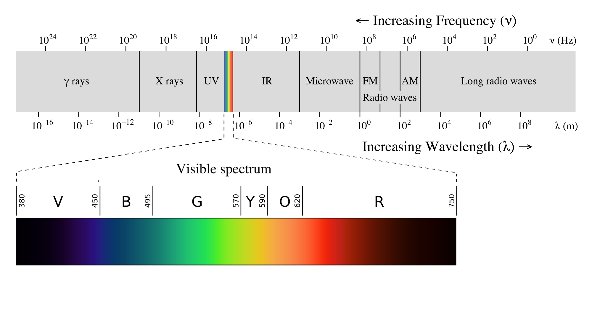
As you can see, electromagnetic waves have a wide variety of uses and effects, dependent on the frequency or wavelength.
Mains electricity is distributed at a frequency of 50 Hz.
Electromagnetic Fields
The electromagnetic phenomena are mediated by the electromagnetic field. This field appears as an electric field, a magnetic field, or a combination depending on your relative movement (in the sense of Einstein's Theory of Relativity). Fortunately, the effects of the electromagnetic field can be separated into separate electric and magnetic fields at the scales relevant to this course.
Electromagnetic fields propagate (or travel) through space.
The speed of light in a vacuum is exactly 299792458 m.s-1. In wires it is a little slower, but the wavelength of 50 Hz electricity is about 6000 km.
This is why we can "get away" with having separate electric and magnetic fields.
The importance of studying electromagnetism comes is for the following reasons:
- charged particles generate electric fields;
- moving charged particles generate magnetic fields;
- time-varying magnetic fields generate electric fields;
- time-varying electric fields generate magnetic fields;
- electric fields exert forces on charged particles;
- magnetic fields exert forces on moving charged particles.
Every one of those points creates a measurable phenomenon, and can be harnessed to transfer energy from one form to another.
2. Vectors and Vector Fields
Electromagnetic fields not only act in time, but also in space.
In particular, electromagnetic fields and forces not only have magnitude ("size", or "strength"), but also direction.
This makes electromagnetic fields vector fields.
Before introducing you to vectors, we must be familiar with scalar is.
Scalars
A scalar is a quantity that has a magnitude or value, but the direction is either meaningless or not important. Scalars include "ordinary" numbers, such as 1 or \( \pi \).
Some examples of scalars:
- time;
- length;
- area;
- volume;
- temperature;
- distance;
- speed;
- acceleration;
- electric charge;
- voltage;
- electric current;
- frequency.
In all these cases, the direction is not important.
Vectors and Vector Fields
See also: Vector (Simple English Wikipedia) :https://simple.wikipedia.org/wiki/Vector.
Vectors differ from scalars in that they have direction. The direction is what makes vectors useful for expressing effects that act in 3D space.
Many electromagnetic phenomena act in 3D space, so vectors are a useful way of expressing electromagnetic phenomena.
Examples of vectors:
- displacement (vector form of length and distance);
- velocity (vector form of speed);
- acceleration (when used as a vector);
- electric field;
- magnetic field;
- force (when used as a vector).
Vectors often occur as a vector field. Vector fields describe the nature of a vector (e.g. gravitational force) in space.
The image below shows an example of Earth's gravitational field, which is a vector field.
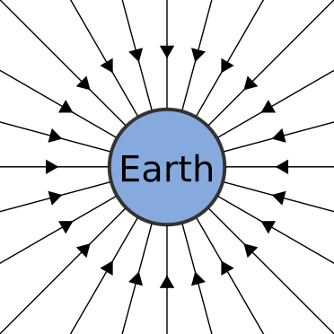
The arrows indicate the direction of Earth's gravitational force vector.
In this case, gravity has the effect of exerting a force that tries to pull an object with mass object towards the centre of the Earth.
3. Electric and Magnetic Fields
This chapter introduces some of the electromagnetic theory associated with electricity.
Some key points from this chapter:
- There are two types of charge: positive and negative. Both charges create electric fields.
- Static (non-moving) charges generate electric fields. These electric fields exert forces on charged particles.
- Electric field forces can be attractive or repulsive.
- Like charges repel, unlike charges attract.
- Magnetic fields are generated by moving charged particles.
- Magnetic fields are generated and can be held indefinitely by certain chemical elements such as iron, nickel and cobalt.
3.1. Electric Fields
Electric fields exert a force on charged particles.
The electric field is a force field with magnitude and direction.
The electric field is a vector field, and its magnitude is usually denoted by the symbol \( E \).
The electric field is important because voltage is the net effect of electric fields.
The electric field has two main physical interpretations:
- the voltage gradient (or change of voltage) with respect to change in distance; or
- the force per unit charge.
In light of the above, the electric field has two main equivalent units:
- volts per metre or V.m-1; or
- newtons per coulomb or N.C-1.
Electric fields are the force that moves electric current around a circuit.
Electric fields are frequently shown using lines or arrows, these arrows show the force on an imaginary positive "test charge".
The test charge will be pushed in the direction of the electric field lines.
The electric field forces might be considered the "true" or "real" electromotive force.
Electric fields have three main sources and behaviours:
- Charged particles: All charged particles create an electric field.
- Time-varying magnetic fields: A time-varying magnetic field will create an electric field that goes in loops.
- Moving a charged particle in a magnetic field: Moving charged particles in a magnetic field creates a force on that charged particle. The ratio of the force to the charge is the strength of the electric field.
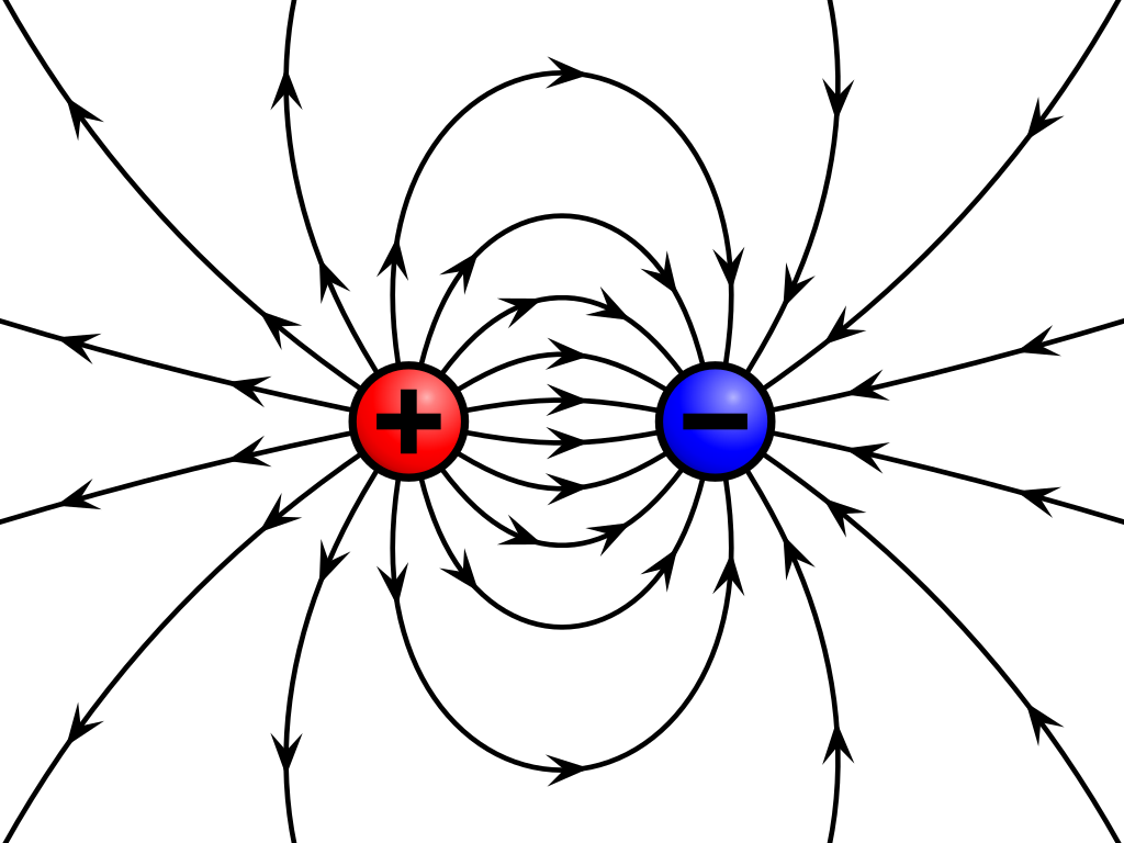
Electric fields are a vector field. Electric fields originate at positively charged particles, and terminate at negatively charged particles. See image below.
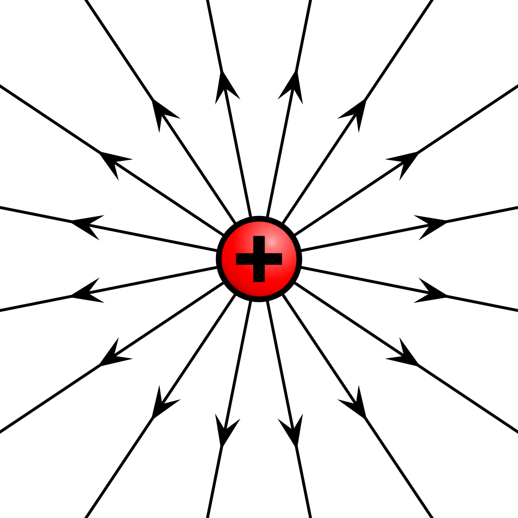
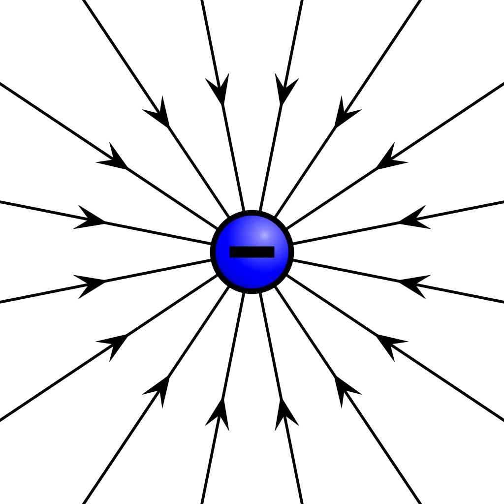
Unlike gravity, which is always attractive, electric field forces can attractive or repulsive.
Like charges repel, and unlike charges attract.
The magnitude of the force from an electric field on a non-moving charge is given by:
\( F = q E \)
where \( F \) is the force (N), \( q \) is the charge (C), and \( E \) is magnitude of the electric field (V.m-1or N.C-1).
The direction of the force is the same as the direction of the electric field.
If a positive charge and a negative charge are brought near each other, the field will look like the one below. It is the sum of the two individual fields. Note that field lines never cross over each other.
Electric Fields and Voltages
Electric fields are not normally measured directly. Normally we measure voltage, which is the sum of electric field strength between two points over a distance.
Voltage has several possible interpretations:
- The total electromotive force that is exerted. This is the origin of calling a voltage an electromotive force (EMF).
- The amount of energy or work that is transferred by each charged particle as it moves through an electric field. In this sense, the unit V is also interpreted as J.C-1 (joule per coulomb). The J unit comes from multiplying force by distance, i.e. 1 J = 1 Nm.
These two units, V and J.C-1, are physically identical.
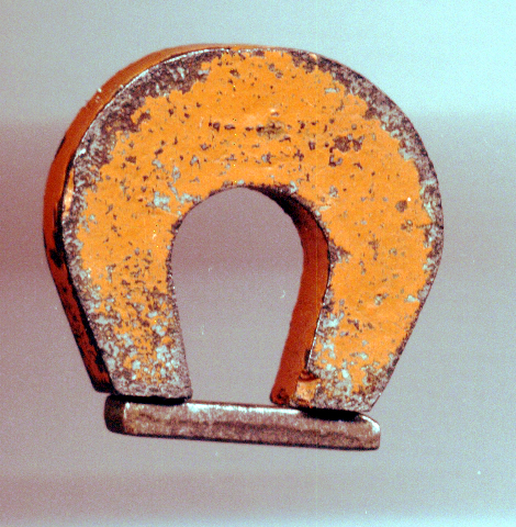
3.2. Magnets
A magnet is any device or object that can produce a magnetic field.
Magnets are two main types:
- permanent magnets: permanent magnets can retain a magnetic field even without an external magnetising force;
- temporary magnets: temporary magnets require an applied magnetising force to create a magnetic field. When the magnetising force disappears, the magnetic field also disappears.
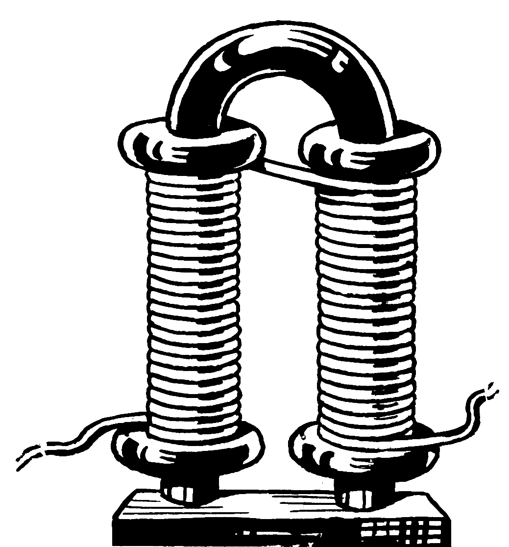
The images below show two types of magnets. The red magnet is a permanent magnet.
The black-and-white image is an electromagnet. An electromagnet uses electric current to generate a temprary magnetic field. The electromagnet image shows a "horseshoe" core with a coil of wire on each "leg".


The magnetic permeability \( \mu \), or permeability describes the magnetic behaviour of a substance. The unit of permeability is the henry per metre, or H.m-1. The henry is the unit of magnetic inductance.
The permeability is the ratio between the magnetic field strength, and the magnetising force.
The magnetic permeability is usually broken into two parts such that \( \mu = \mu_0 \mu_{\mathrm{r}} \).
The two parts are:
- \( \mu_0 \): the permeability of free space. The permeability of free space (or a vacuum) is a fundamental constant of the universe. The permeability of free space has the approximate (since 2019, but still accurate to better than 1 part in a billion) value of \( 4\pi \cdot 10^{-7} \) H.m-1. The numerical value is \( 1.2566 \cdot 10^{-7} \) H.m-1.
- \( \mu_{\mathrm{r}} \): the relative permeability, the ratio of the permeability of the substance of interest to the permeability of free space.
Magnetic materials have a relative permeability (\( \mu_{\mathrm{r}} \)) greater than 1. Materials that have high permeability are called ferromagnetic or ferrimagnetic materials, depending exactly how they achieve their high permeability.
Not many materials than iron, nickel, cobalt or their compounds and alloys have a relative magnetic permeability significantly more than 1. Most other substances can be treated like free space (i.e. \( \mu_{\mathrm{r}} = \) 1 ).
3.3. Magnetic Fields
The magnetic field is a vector field that exists in all regions of space.
Humans lack any direct means of detecting magnetic fields, but magnetic fields can be detected by observing their effects on other magnets or magnetically permeable substances.
An example is a compass. A compass contains a bar magnet that aligns itself with Earth's magnetic field.
Compasses also work with any other magnetic field.
Another effective means of seeing a magnetic field is with iron filings. Iron filings are a fine iron powder that can be sprinkled around magnets.
The image below shows iron filings sprinkled on a sheet of paper placed over a bar magnet.
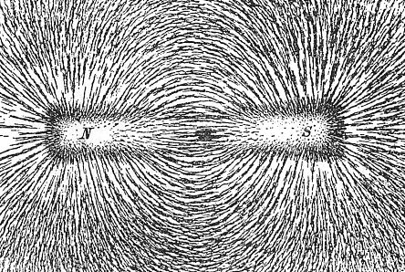
The iron filings align themselves along the magnetic field in lines. These lines are the shape of the magnetic field.
Iron filings do not give the direction of the magnetic field. In the illustration above, it is not possible to tell which pole is which by the iron filings alone. A compass must be used to determine the direction. The "north" end of the compass needle points in the direction of the magnetic field.
The closer the iron filings are to each other, the stronger the magnetic field.
Every magnet has two poles, a north pole, and a south pole. The magnetic poles are where the field lines appear to "leave" and "enter" the magnet.
Magnetic poles are also where the magnetic field lines are the most concentrated as they leave (or enter) a magnet.
In a bar magnet, the poles are at the ends. The poles is also the area where the magnetic flux density is the greatest, as the iron filings are the most concentrated there.
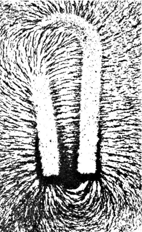
The picture below shows the magnetic field of a horseshoe magnet. Note how strong the magnetic field is at the poles, as they are closer together than with a bar magnet.
Magnetic Fields and Magnetic Flux
The magnetic field is a vector quantity. The magnitude of the magnetic field has the symbol \( B \). The unit of magnetic field is the tesla or T.
The magnetic field may also be defined as the magnetic flux density; or magnetic flux per unit area.
The magnetic flux represents the total magnetic field \( B \) over an area.
The unit of magnetic flux has three interpretations: the weber (Wb), the tesla metre squared (T.m2), or the volt second (Vs). Note that 1 T = 1 Wb.m-2.
The magnetic field may also be represented as magnetic flux, with the symbol \( \Phi \) (Greek letter capital 'phi').
Magnetic fields are vector fields like electric fields, but with an important difference: there are no net "sources" or "sinks" of magnetic fields.
In other words, magnetic field lines do not "start" at a north pole, and "terminate" at a south pole. Magnetic field lines are always closed loops, with no start and no end.
The picture below shows the simplest magnetic field: a magnetic dipole.
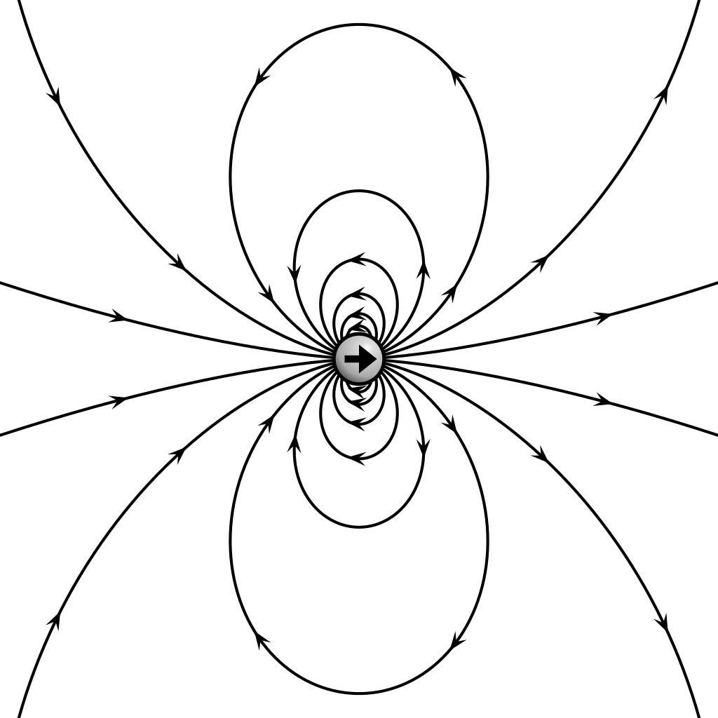
Outside the magnetic object, the magnetic field lines point towards the south pole, and come away from the north pole.
Note how all the field lines form closed curves. The south pole is on the left of the dipole, the north pole is on the right. The closer the lines are to each other, the stronger the field.
Behaviour of Magnets and Magnetic Fields
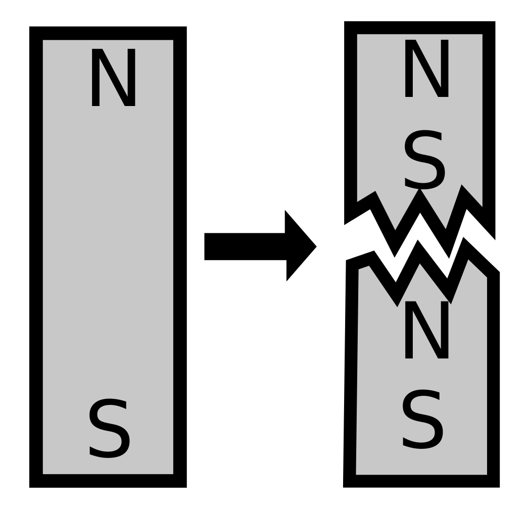
For a permanent magnet, every atom is a magnetic dipole. That means that if you cut a magnet in half, you will not get a separate north and south pole.
You will get two magnets, each with their own north and south poles.
Magnetic field direction is commonly detected using another magnet, e.g. a compass. The illustration below shows how this is done using compasses. The compass points in the direction of the magnetic field. As can be seen below, the magnetic field lines go from the north pole to the south pole. In other words, south sucks".
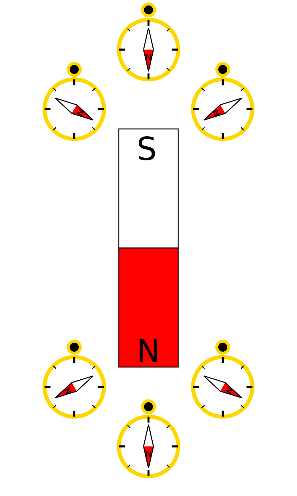
Compasses were originally designed to detect magnetic north. The compass needle itself is a small magnet. The part of a compass needle that points north is a magnetic north pole. The needle gives the direction of the magnetic force, the magnetic field going in the direction the compass needle is pointing. Note that this means that the compass needle always points towards a south pole. The magnetic pole in Earth's northern hemisphere is actually a south pole!
Magnetic Attraction and Repulsion
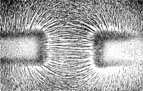
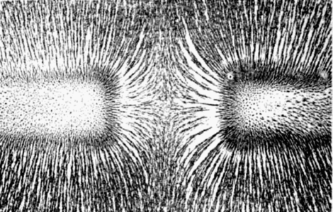
Magnets are capable of interacting with each other. The images below show two situations: attraction between unlike poles, and repulsion between like poles.
The image below shows magnetic attraction. The iron filings in the middle go pretty much straight from one magnet to another. These magnets may also produce a noticeable force, and may actually pull themselves together so they are touching.
The image below shows magnetic repulsion. The iron filings in the middle are quite sparse, and the field lines look "squeezed outwards" with a "dead spot" in the centre between the magnetic poles. These magnets may also produce a noticeable force, and may actually push themselves apart.
3.4. Magnetising Force
Magnets and magnetic substances respond to a magnetising force.
Magnetising force is represented by \( H \), and has the unit A.m-1. The relationship between magnetising force \( H \) and flux density \( B \) for "soft" magnetic materials is described by:
\( B = \mu H = \mu_0 \mu_{\mathrm{r}} H \)
where \( B \) is the magnetic field (T), \( \mu \) is the magnetic permeability (H.m-1), and \( H \) is the magnetising force (At.m-1).
The magnetising force is provided by passing current through a wire or similar. The unit has the value amp-turns per metre, in the sense that the magnetising force is amplified by the number of turns of a coil of wire. Physically the unit is the same as A.m-1.
The unit henry is the ratio of magnetic flux to current i.e. 1 H = 1 Wb.A-1. So the higher the permeability, the stronger the magnetic flux you can create for a given amount of current.
Every material has its own response of magnetic field to magnetising force. Two types of magnetic materials are shown below.
Hard and Soft Magnetic Materials
The response of a magnetic material to a magnetising material is described using a B-H curve.
The material on the left is a soft magnetic material.
The reason is the it takes a relatively small value of \( H \) is required to reverse the magnetic field.
Soft magnetic materials are excellent when the magnetic field is changed frequently, such as in transformers.
Soft magnetic materials are a poor choice for permanent magnets, as the residual magnetic field is weak.
In contrast, a hard magnetic material requires a high value of \( H \) to reverse the magnetic field.
Hard magnetic materials are excellent when the magnetic field needs to be retained, such as in permanent magnets.
Hard magnetic materials are a poor choice when the magnetic field is changed frequently, such as in transformers.
The image below shows two B-H curves. The one on the left is for a soft magnetic material, the one on the right is for a hard magnetic material.
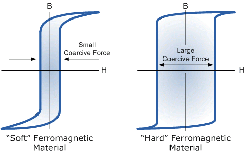
Another notable feature is the levelling of of the curve at high values of positive or negative \( H \). This is called magnetic saturation, and results in a drop in permeability. Most electrical steels saturate at a flux density of 1.2-2.2 T.
3.5. Permanent (Hard) Magnets
Permanent magnets are capable of holding a permanent magnetic field. Many of these materials are ferromagnetic, in the sense that they use ferromagnetism to hold their magnetic field. Most common magnetic materials such as iron, nickel, cobalt and their alloys are ferromagnetic.
Permanent magnets are usually made of "hard" magnetic materials, in the sense that:
- hard magnetic materials retain their magnetic field after an external field is removed; and
- hard magnetic materials are difficult to magnetise and de-magnetise using an external magnetic field.
Hard magnetic materials are useful in:
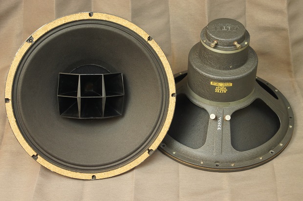
- permanent magnets, such as in loudspeakers, fridge magnets, actuators, dc motors;
- information storage such as swipe cards and hard drives.

3.6. Temporary (Soft) Magnets
Temporary magnets are usually made of "soft" magnetic materials, in the sense that:
- soft magnetic materials lose their magnetic field after an external field is removed; and
- soft magnetic materials are easy to magnetise and de-magnetise using an external magnetic field.
Any substance (including free space with \( \mu_{\mathrm{r}} = 1\)) is technically a soft magnet, but the term usually refers to magnetic materials (high permeability) that can have their magnetisation easily changed. Common examples of soft magnetic materials include transformer steel, silicon steel and soft iron.
Soft magnetic materials are useful in:
- transformers, because soft magnetic materials produce lower losses;
- iron filings used to see magnetic fields; and
- lifting magnets, bells, contactors, relays, solenoids, and locking magnets, where the holding force needs to disappear when the current is turned off.
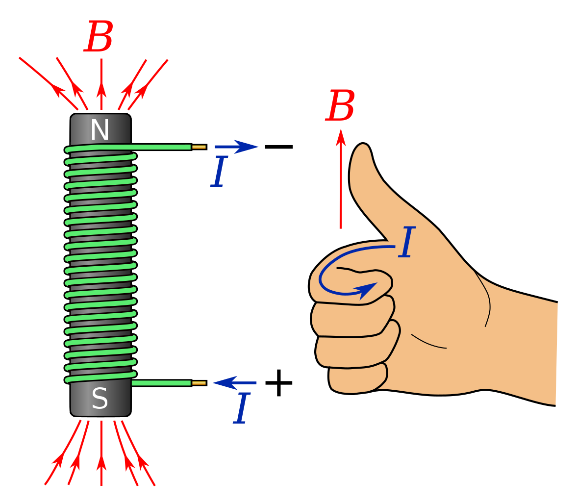
Electromagnets
A coil of wire can be used to generate a controllable magnetic field by varying the current flow in the coil. This type of magnet is called an electromagnet, solenoid or coil. A solenoid with a U-shaped core is shown below.
Magnetising Force
The magnetising force \( H \) is given by the equation:
\( H = \frac{N I}{l} \)
where \( H \) is the magnetising force (A.m-1), \( I \) is the magnetising current (A), \( l \) is the total effective length of the magnetic circuit (m), and \( N \) is the number of turns.
In the case of the electromagnet above, the magnetic circuit length is the length all the way from the end of one coil, through the pole piece, through the end of the other coil, and back to the end of the first coil.
Transformers
Another common electromagnet is the transformer. The magnetic circuit is through the transformer core, which for efficiency has a permeability as high as possible.
The primary winding is used to generate a magnetising force that ends up generating an EMF in the secondary winding.

B-H Curves
The most important curve when designing electromagnets is the B-H curve. A set of B-H curves are shown below for various types of steels. Note the levelling off of the curve of B-H at about 1-2 T. This is the effect of magnetic saturation.
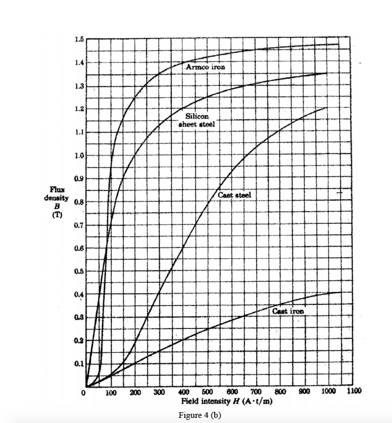
The curves are determined experimentally for each material. The slope of the curve is the value of \( \mu \) at that particular magnetising field strength.
The "average" permeability is given by \( \frac{B}{H} \). The "average" relative permeability is given by \( \frac{B}{\mu_0 H} \).
The horizontal axis is in "amp-turns per metre". The meaning of this is that if you need 500 amp-turns, you could get that magnetising force in any one of the following ways:
- 1 turn of wire carrying 500 A;
- 5 turns of wire carrying 100 A;
- 100 turns of wire carrying 5 A;
- 500 turns of wire carrying 1 A;
- or any other combination of turns and current such that the product \( N I \) is 500.
Electromagnet Forces
Electromagnets are capable of producing a physical force on magnetisable materials. The force is given by:
\( F = \frac{B^2 A}{2 \mu_0} \)
where \( F \) is the force (N), \( B \) is the magnetic field (T), \( A \) is the area of the magnetic circuit (m2), and \( \mu_0 \) is the magnetic permeability of free space (H.m-1).
The value of \( B \) at a particular value of \( H \) is obtained by reading a B-H curve like the one above.
4. Electromagnetic Effects
4.1. Magnetic Fields of Single Wires and Coils
Moving charges create a magnetic field. In particular, an electric current flowing in a wire generates a magnetic field.
The law that describes the Biot-Savart Law (bee-o savar).
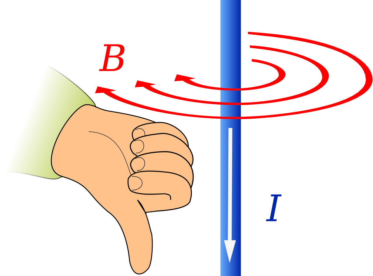
Right-Hand Grip Rule (Side-On)
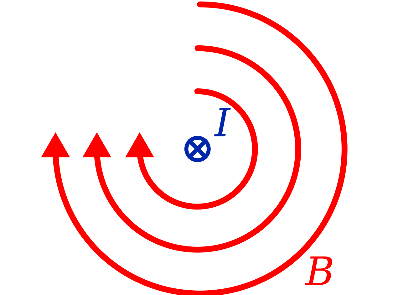
A current in a particular direction in a long, straight wire will generate a circular magnetic field, as shown below.
The direction of the magnetic field is given by the right-hand grip rule.
A current flowing in the direction shown by your thumb will generate a magnetic field that curls in the same direction as your fingers. Two "side on" views are shown below, with the way the right hand showing the direction of the field lines.
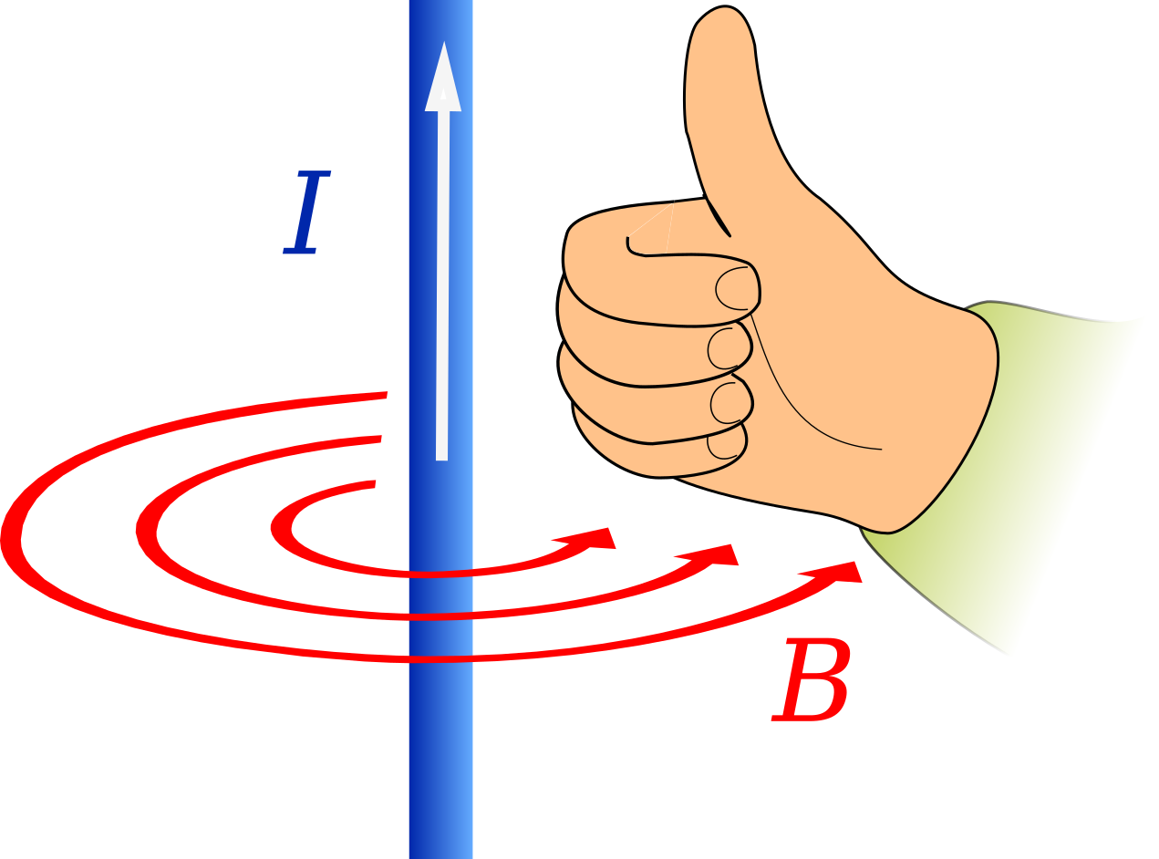
The magnetic field lines depend directly on the direction of the current. If the direction of current is reversed, the magnetic field lines also reverse direction.
Calculating the Magnetic Field Around a Single Wire
The magnitude of the magnetic field around a long, straight wire is given by:
\( B = \frac{\mu_0 \mu_{\mathrm{r}} I}{2 \pi r} \)
where \( B \) is the magnetic field (T), \( \mu_0 \) is the permeability of free space, \( \mu_{\mathrm{r}} \) is the relative permeability, I is the current (A), and \( r \) is the radial distance from the centre-line of the wire (m).
For the magnetic field of a wire in air, \( \mu_{\mathrm{r}} = \) 1.
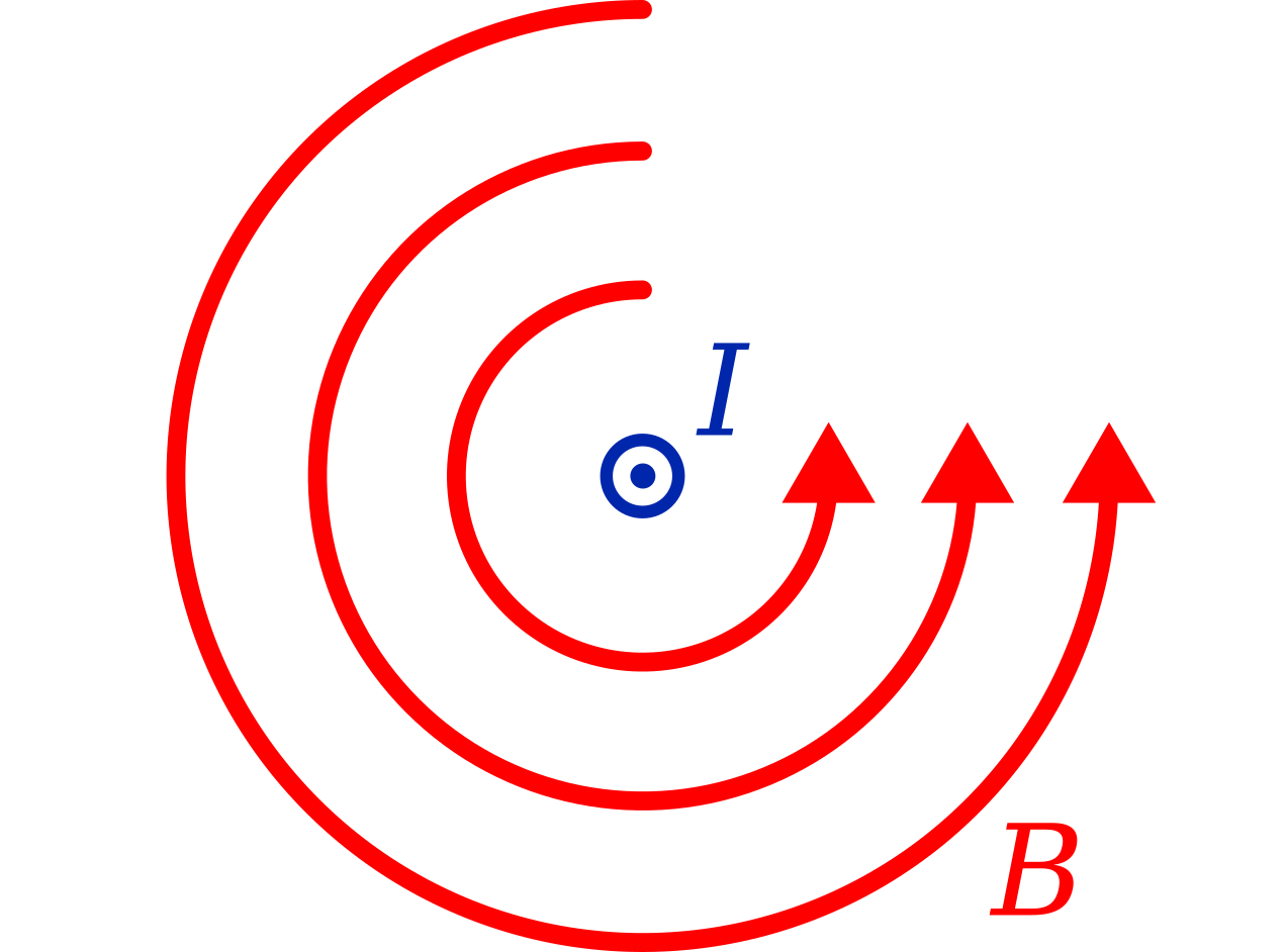
Right-Hand Grip Rule (End-On)
The direction of the current and magnetic field can also be shown "end on".
The current is thought of as going either directly towards you, or directly away from you.
The symbol is chosen by analogy with an arrow.
The symbol "\( \odot \)" means the current is flowing towards you.
The symbol "\( \otimes \)" means the current is flowing away from you.
The two images below show the magnetic fields around the wires with these different directions of current.
Current going towards you (\( \odot \)). Your thumb points towards you. The fingers on your right hand will curl anticlockwise as you look at them.
Current going away from you (\( \otimes \)). Your thumb points away from you. The fingers on your right hand will curl clockwise as you look at them.
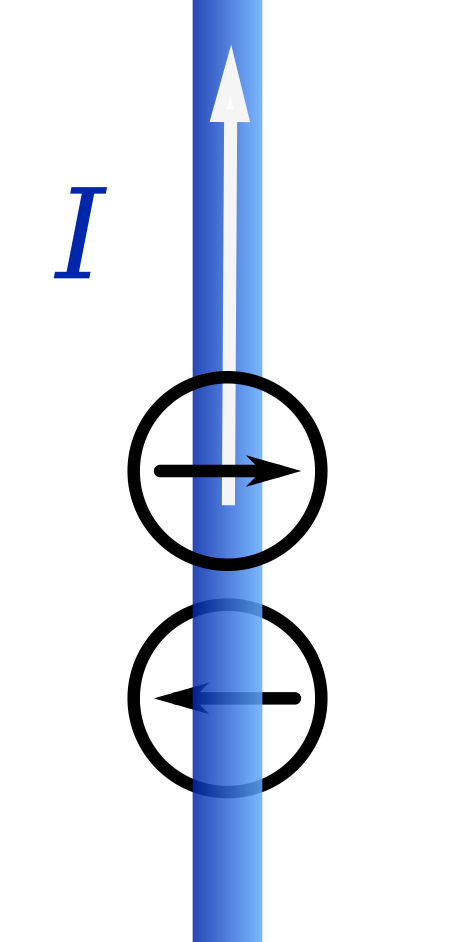
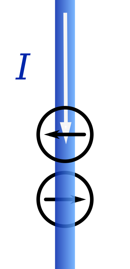
Observing the Magnetic Field Around a Wire (Side-On)
It is possible to use a compass to see the magnetic field around a current-wire.
The compass needle will be deflected as shown below.
The compass needle is always at right angles to the wire (notwithstanding any other strong magnetic fields that might disturb the compass needle).
The two images below show two compasses. One compass is placed below the wire, and the other compass is placed above the wire. The compass needles will point in the directions shown.
Since the magnetic field is circular, compasses placed on opposite sides of the wire will point in opposite directions.
The directions themselves are predicted using the right-hand rule.
The needle directions for the current travelling "upwards" is shown below.
The needle directions for the current travelling "downwards" is shown below.
Observing the Magnetic Field Around a Wire (End-On)
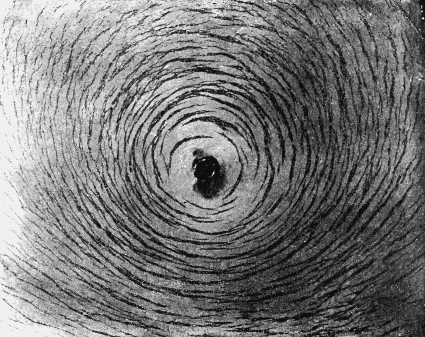
The magnetic field around a wire can be observed by various means, including:
- placing iron filings on a sheet of paper at right angles to the wire; and
- using compasses.
The magnetic field is circular, with the direction given using the right-hand rule.
The picture below shows iron filings placed on a sheet of paper with a current carrying wire passing through it. The filings are aligning themselves in rings.
placing compasses around a current-carrying wire, like in the diagram below. The wire is carrying current directly towards you. The compasses show the direction of the magnetic field around the wire.
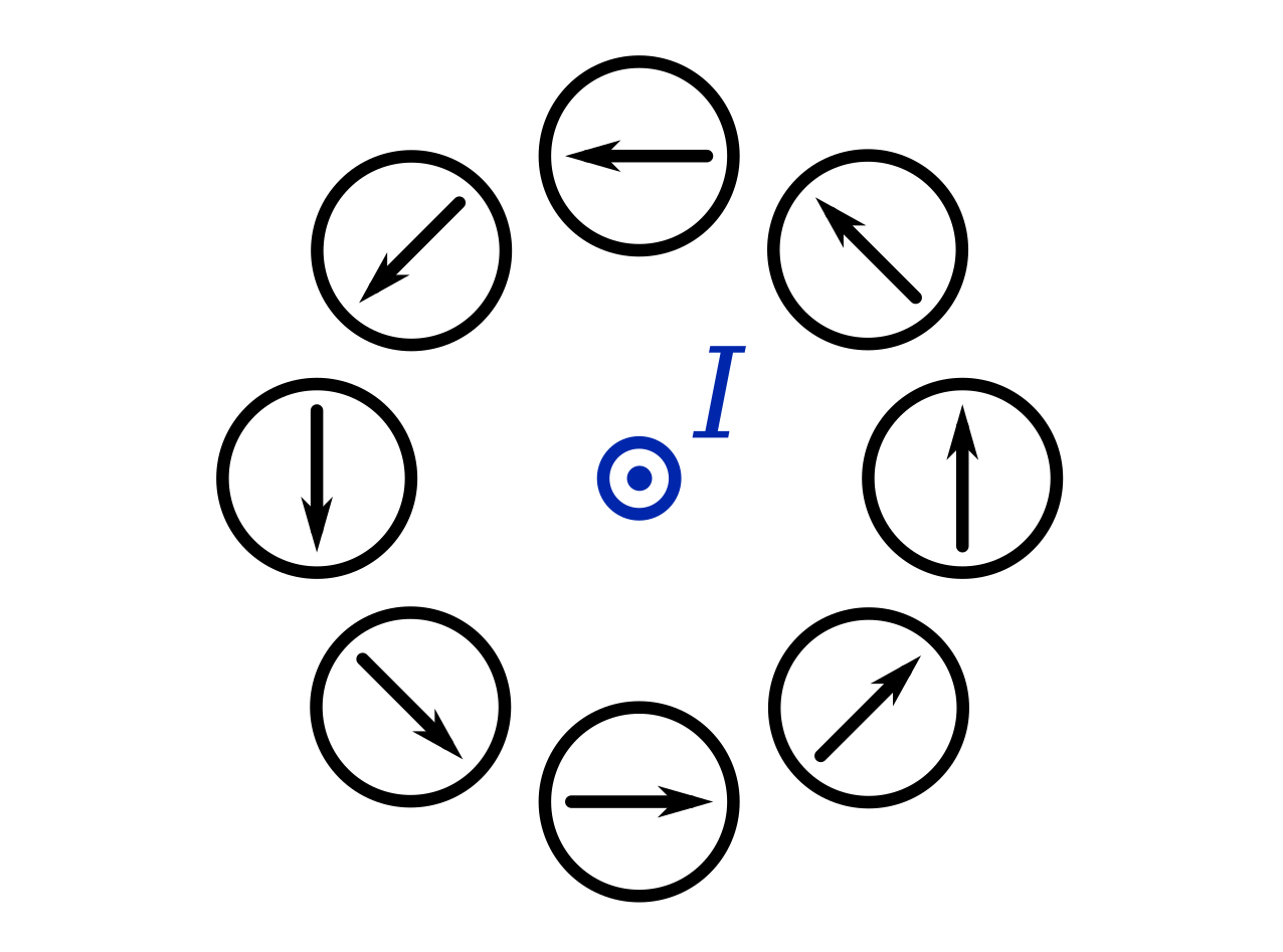
The same diagram for a current going away from you is shown below.

Magnetic Fields of Electromagnets
The direction of the magnetic field of an electromagnet is found using the right hand grip rule in reverse.
The fingers curl in the direction of the current, and the thumb points in the direction of the magnetic field in the centre of the coil. Or, as shown below, the thumb points towards the north pole.
Another way of viewing the magnetic field is to look at the solenoid in section as below. The solenoid has been "cut in half" lengthwise, so that every turn can be seen.
The dots represent a current coming towards you, and the crosses represent the current going away from you.
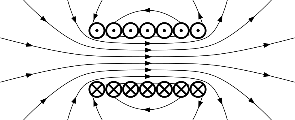
The magnetic field shown is the sum of the fields from each wire. The directions can be verified using the right hand grip rule on each turn, and checking they are the same as the direction of the total field.
Another method of remembering the magnetic poles in an electromagnet is shown below.
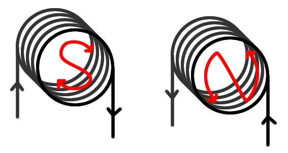
If the current flow is clockwise at the end of the coil, then the pole is a south pole at that end. If the current flow is anticlockwise at the end of the coil, then the pole is a north pole at that end.
NOTE: It is important to not confuse the direction of the current flow with the direction the coil is wound. The direction of current flow depends on the polarity of the voltage applied to the coil and the direction the coil is wound.
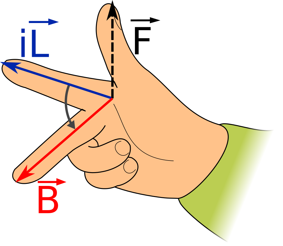
4.2. Force Between a Current-Carrying Wire and a Magnet
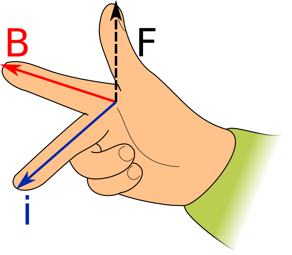
Any current-carrying conductor that is in a magnetic field will experience a physical force.
The force will be at right angles to both the current, and the magnetic field.
The force on a current-carrying conductor in a magnetic field is given by:
\( F = B i L \sin \theta \)
where \( F \) is the magnitude of the physical force on the wire (N), B is the magnetic field (T), i is the current, L is the length of the conductor in the magnetic field (m), and \( \theta \) is the angle between the length and magnetic field vectors.
If the current and magnetic field are parallel (going in the exact same direction) or anti-parallel (going in exact opposite directions), the force is zero. This is because \( \theta = \) 0° (parallel) or \( \theta = \) 180° (anti-parallel).
The force magnitude is a maximum when the current and magnetic field are at right angles to each other.
The force is always perpendicular (at right angles) to both the magnetic field and direction of current flow.
The rules below explain how the force direction is determined.
Determining the Direction of the Magnetic Force
There are many ways of determining the direction of the magnetic force.
Four common ways are presented below.
The right-hand rule, left-hand rule, and right-hand slap rule work by examining the effect of the magnetic field directly on the current-carrying conductor.
The hands-free method works by noting that while for force is always directly on the current-carrying conductor itself, the direction of the force can also be determined by seeing the effect a current has on the local magnetic field.
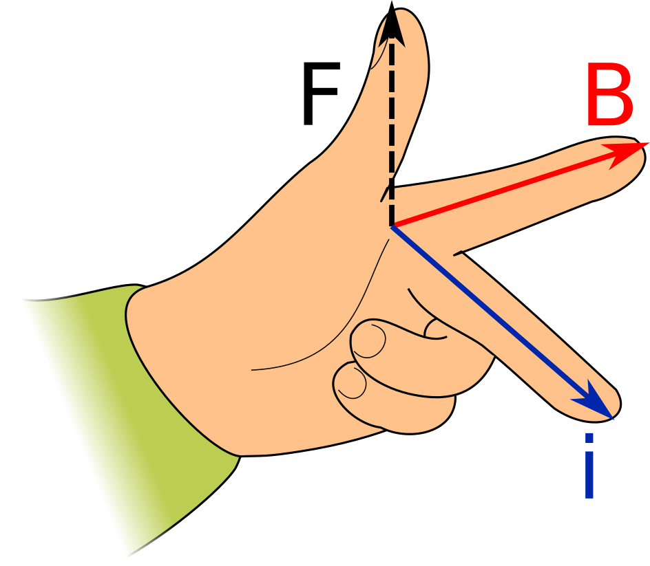
Right-Hand Rule
The direction of the force is given using the right-hand rule, as shown below.
Left-Hand Rule
Some sources may describe the direction of the force using the left-hand rule, as shown below. The left-hand rule is similar to the right hand rule, except that it uses the left hand, and the current and field are swapped between the index
and middle fingers.

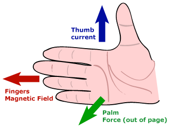
Right Hand Slap Rule
The right-hand slap rule or right-hand palm rule is shown below.
The thumb represents the direction of the current. The fingers represent the magnetic field.
The direction of the force is the direction you would move your right hand as if you were trying to slap an object.
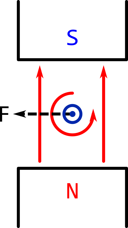
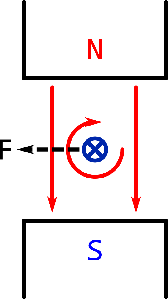
Analysing the Magnetic Field ("Hands-Free Method")
A wire in a magnetic field will always be pushed from the stronger magnetic field to the weaker magnetic field.
This means the direction of force can be determined without using any hand rules.
Consider a current carrying wire in a magnetic field, as shown below. The force on the wire is shown pointing to the right. The reason for this is explained below.
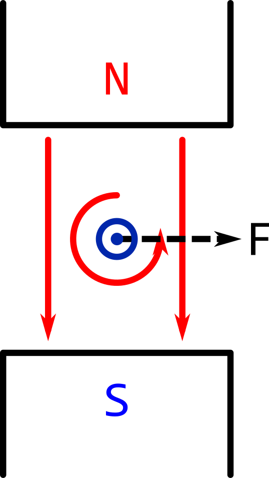
The drawing shows parts of two magnetic fields: one from the permanent magnet, and the other from the current-carrying wire.
The magnetic field from the wire is circular and anti-clockwise.
The magnetic field from the permanent magnet is straight down.
On the left, the magnetic field from the wire strengthens the total magnetic field, because both magnetic fields are pointing in the same direction.
On the right, the magnetic field from the wire weakens the total magnetic field, because the magnetic fields are pointing in opposite directions.
The force is along the line that weakens the total magnetic field the most quickly.
In the case of the picture above, the force is to the right.
Swapping the direction of the current and the direction of the magnetic field at the same time will not affect the direction of the force.
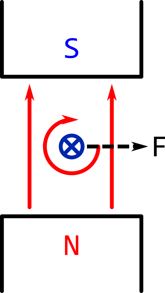
Swapping one of the current direction or the magnetic field direction will reverse the direction of the force.
Another "swapped" scenario is shown below.
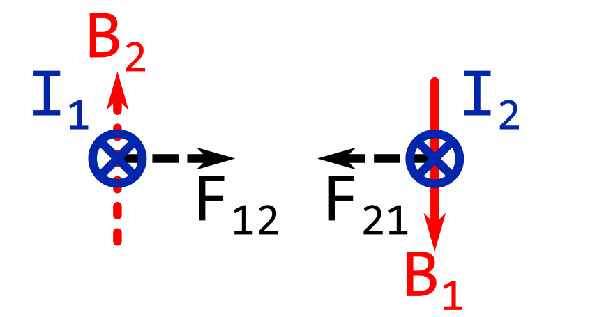
4.3. Force Between Two Current-Carrying Conductors
As noted previously, a current-carrying conductor in a magnetic field experiences a force given by:
\( F = B i L \sin \theta \).
So far, a permanent magnet has been considered as the source of that magnetic field.
However, it is possible for the source of the magnetic field to be another current-carrying wire.
In this course, we will consider the force between parallel current-carrying wires.
If the wires are parallel, the magnetic field from one wire passing through another will always be at right angles.
Therefore, the equation for the force can be simplified to:
\( F = B i L \).
Analysis
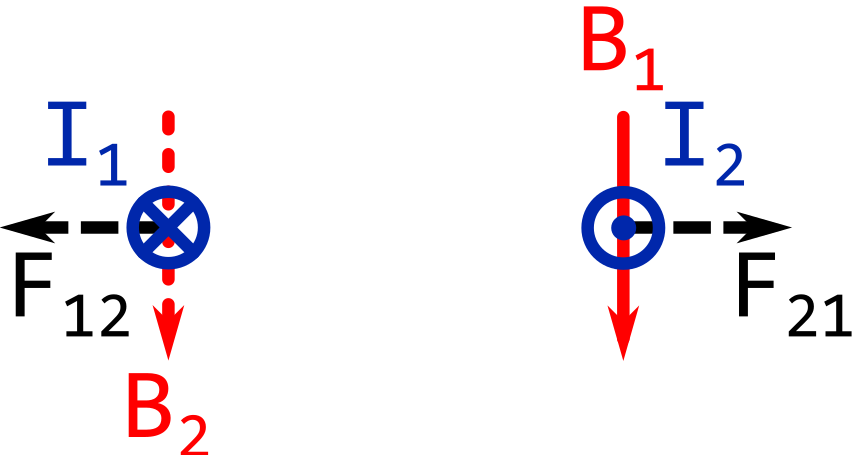
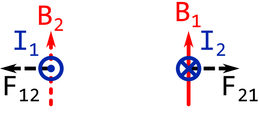
The images show two long, parallel wires. The \( \otimes \) and \( \odot \) symbols represent the current going into or coming out of the screen surface respectively.
Since there are two wires, there are two sets of magnetic fields.
Note that a given conductor is not affected by its own magnetic field. The force comes from the combination of the conductor's current and the other conductor's magnetic field.
| Description | Symbol - Conductor 1 |
Symbol - Conductor 2 |
|---|---|---|
| Force on a particular conductor (N) |
\( F_{12} \) |
\( F_{21} \) |
| Magnetic field due to that particular conductor (T) |
\( B_1 \) |
\( B_2 \) |
| Current in a conductor (A) |
\( i_1 \) | \( i_1 \) |
The conductors are spaced \( d \) metres apart (not shown on the drawings).
If the currents in the wires are going in the same directions, the wires will attract each other.
The image below shows both currents going away from you.
The image below shows both currents going towards you.
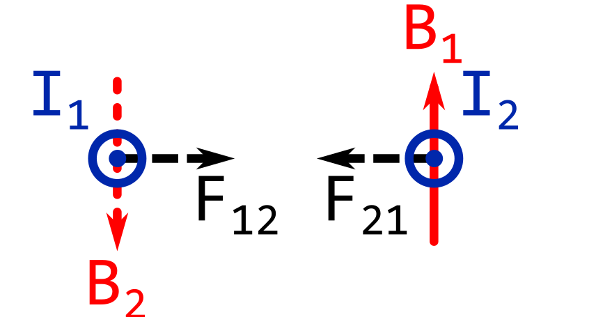
If the currents in the wires are going in the opposite directions, the wires will repel each other.
The image below shows \( I_1 \) going away from you.
The image below shows \( I_1 \) going towards you.
The force between the conductors is mutual. The conductors are pushed away from (or pulled towards) each other.
It is easier to see the force when the wires start moving when the current is first applied.
The first "half swing" will tell you whether the nature of the force.
If the wires swing away from each other, the force is repulsive. If the wires swing towards each other, the force is attractive.
Force Calculation
The basic equation for the force is:
\( F = B i L \)
But the magnetic field is known, as it comes from the other conductor.
The magnetic field around a long, straight current-carrying conductor is given by:
\( B = \frac{\mu_0 \mu_{\mathrm{r}} i}{2 \pi d} \)
where \( B \) is the magnetic flux density (T), \( \mu_0 \) is the permeability of free space (H.m-1), \( \mu_{\mathrm{r}} \) is the relative permeability of the medium surrounding the conductor (dimensionless), \( i \) is the current through the conductor (A), and \( d \) is the radial distance from the conductor (m).
Given that \( \mu_0 \) is approximately (to about 1 part in 1 billion) \( 4 \pi \cdot 10^{-7} \), the magnetic field equation can be simplified further.
\( B = 2 \cdot 10^{-7} \cdot \frac{\mu_{\mathrm{r}} i}{d} \)
The force seen by conductor 1 is:
\( F_{12} = B_2 i_1 L = 2 \cdot 10^{-7} \cdot \frac{\mu_{\mathrm{r}} i_1 i_2}{d} \)
The force seen by conductor 1 is:
\( F_{21} = B_1 i_2 L = 2 \cdot 10^{-7} \cdot \frac{\mu_{\mathrm{r}} i_1 i_2}{d} \)
Note these forces are both the same magnitude.
If the current in both wires is the same, the force equation simplifies to:
\( F = 2 \cdot 10^{-7} \cdot \frac{\mu_{\mathrm{r}} i^2}{d} \)
For wires suspended in air, the forces are fairly small, and care is needed to observe the force.
For example, suppose two 1 m long wires are suspended 0.1 m apart in air (\( \mu_{\mathrm{r}} = \) 1), and are carrying 10 A in opposite directions.
The force is calculated below.
\( F = 2 \cdot 10^{-7} \cdot \frac{i^2 L}{d} = 2 \cdot 10^{-7} \cdot \frac{10^2}{0.1} = \) 0.0002 N.
Since the currents are flowing in opposite directions, the force is repulsive. Note that the force is quite small. The force is the same as the weight of an item with a mass of 20.3 µg.
The forces are made larger with higher permeability magnetic materials, having multiple turns of wire, and closer spacings.
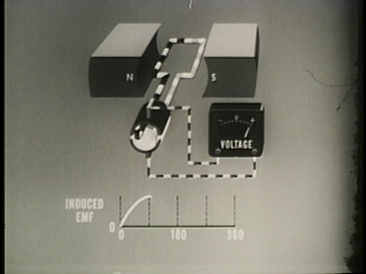
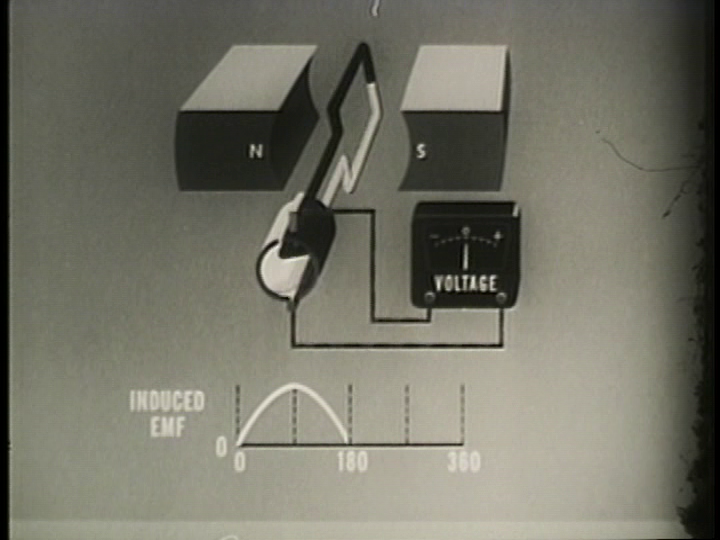
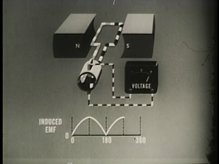
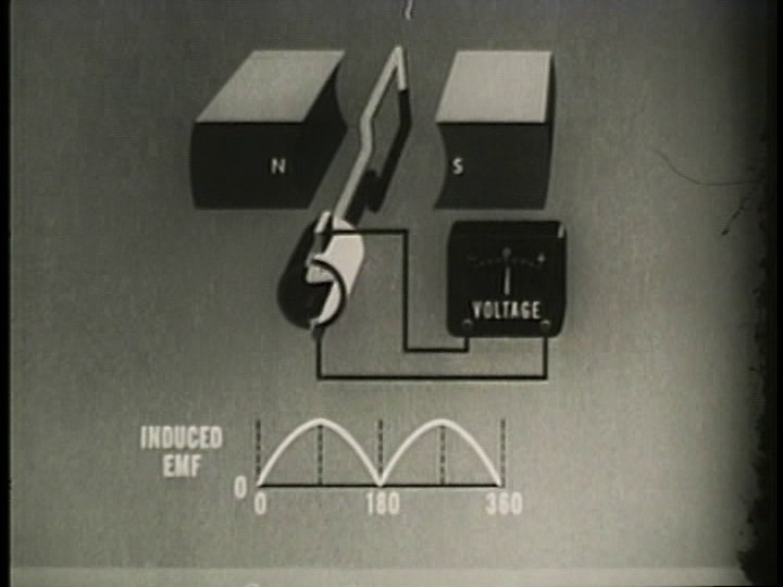
4.4. Electromagnetic Induction in Stationary Coils and Transformers (Faraday's Law)
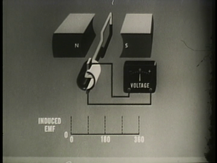
Faraday's Law of Induction relates an electromotive force generated in a length of wire to the rate of change of the magnetic flux passing through the coil with respect to time.
The changing magnetic flux generates a curled electric field i.e. an electric field that goes in loops. Using a wire (or a coil) captures this looped electric field, generating an EMF.
Faraday's Law of Induction is:
\( \mathcal{E} = -N \frac{\Delta \Phi}{\Delta t} \)
where \( \mathcal{E} \) is the electromotive force (V), N is the number of turns of the coil (dimensionless), and \( \Phi \) is the magnetic flux passing through the coil (Wb). The quantity \( \frac{\Delta \Phi}{\Delta t} \) represents the rate of change of the magnetic flux with respect to time (Wb.s-1 or V).
The EMF is negative because it always tries to oppose the change in magnetic field.
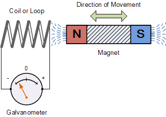
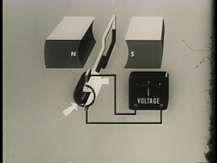
The picture below shows an example of this phenomenon. The magnet is moving, subjecting the coil to a changing magnetic flux. This changing magnetic flux causes an EMF to be induced in the coil, making the needle on the galvanometer move.
The EMF can also be related to the magnetic flux density, if the area of the coil is known. This form is shown below.
\( \mathcal{E} = -N A \frac{\Delta B}{\Delta t} \)
where \( \mathcal{E} \) is the electromotive force (V), N is the number of turns of the coil, \( A \) is the enclosed area of the coil, and \( B \) is the magnetic flux density (T). The quantity \( \frac{\Delta B}{\Delta t} \) represents the rate of change of the magnetic flux density with respect to time (T.s-1).
Transformers
Transformers make use of Faraday's Law of Induction. An illustration of a transformer is shown below.
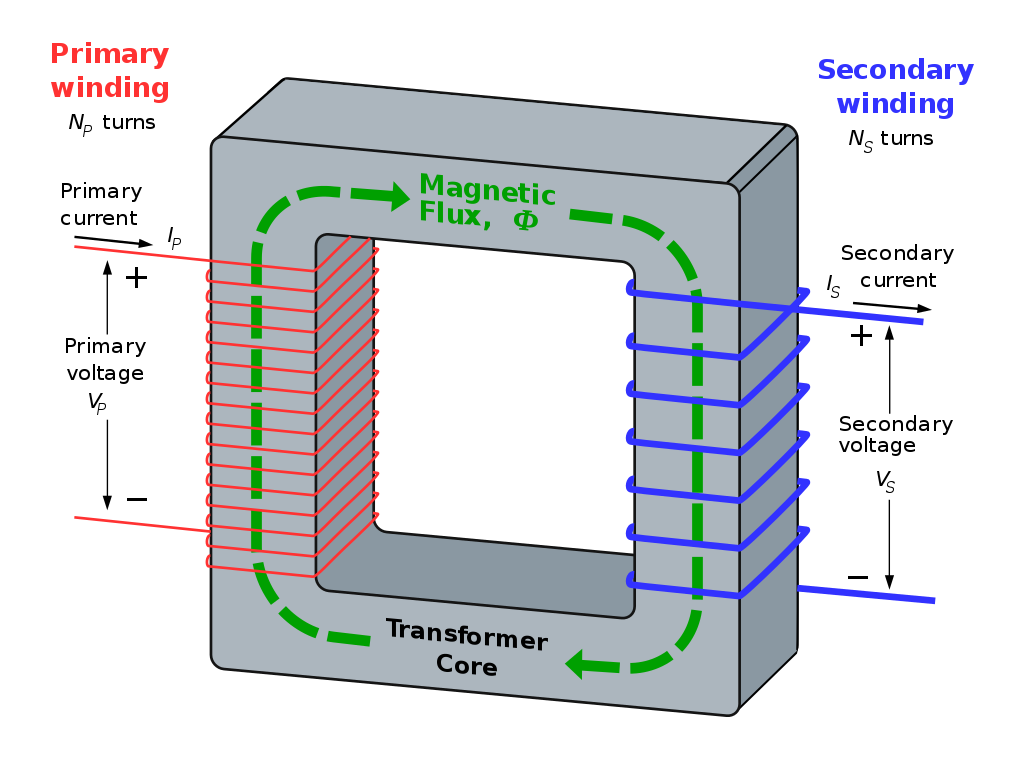
The current flowing through the primary winding generates a magnetic flux \( \Phi \). The magnetic flux travels through the high-permeability core, and intercepts the secondary winding.
If the magnetic flux is changing, an EMF (the secondary voltage) will be generated in the secondary coil.
The induced EMF in the secondary coil can be used to power a load.
The advantages of transformers are the following:
- they can change voltages and currents i.e. they can step-up or step-down voltages and currents;
- there is no electrical contact required between the primary and secondary i.e. transformers can provide electrical isolation.
The ability to electrically isolate the primary and secondary is a major safety benefit.
The secondary voltage can be changed by varying the number of turns on the secondary winding.
Transformers are not DC devices. Operating a transformer at DC would require two things:
- unlimited magnetic flux; and
- windings without any resistance.
While it is possible to use super-conductors with zero resistance for the windings, it is not possible to have unlimited magnetic flux. In practice, transformers can only be used with alternating current.
Calculating Transformer Voltages and Currents
Assuming the resistance of a transformer winding is small (so that any primary resistance causes a small voltage drop due to primary current \( I_{\mathrm{p}} \), the rate of change of flux on the primary coil is the same as the primary voltage \( V_\mathrm{p} \).
\( V_{\mathrm{p}} = -N_{\mathrm{p}} \frac{\Delta \Phi_{\mathrm{p}}}{\Delta t} \)
On the secondary side, a similar situation applies.
\( V_{\mathrm{s}} = -N_{\mathrm{s}} \frac{\Delta \Phi_{\mathrm{s}}}{\Delta t} \)
Note that the secondary voltage is dependent on \( \Phi_{\mathrm{s}} \), the magnetic flux passing through the secondary. In a "good" transformer, the secondary flux will be nearly the same as the primary flux, so \( \Phi_{\mathrm{s}} \) can be replaced with \( \Phi_{\mathrm{p}} \).
\( V_{\mathrm{s}} = -N_{\mathrm{s}} \frac{\Delta \Phi_{\mathrm{p}}}{\Delta t} \)
This allows us to derive a relationship between the primary and secondary voltages.
\( \frac{V_{\mathrm{p}}}{V_{\mathrm{s}}} = \frac{-N_{\mathrm{p}} \frac{\Delta \Phi_{\mathrm{p}}}{\Delta t}}{-N_{\mathrm{s}} \frac{\Delta \Phi_{\mathrm{p}}}{\Delta t}} = \frac{N_{\mathrm{p}}}{N_{\mathrm{s}}} \)
\( V_{\mathrm{s}} = \frac{N_{\mathrm{s}}}{N_{\mathrm{p}}} V_{\mathrm{p}} \)
The primary and secondary currents are calculated by observing that the magnetising forces from the primary and secondary windings must balance.\( H_{\mathrm{p}} = k N_{\mathrm{p}} I_{\mathrm{p}} \)
\( H_{\mathrm{s}} = k N_{\mathrm{s}} I_{\mathrm{s}} \)
The value \( k \) depends on the exact details of the transformer construction, but it is assumed that \( k \) is the same for both primary and secondary windings.
\( \frac{H_{\mathrm{p}}}{H_{\mathrm{s}}} = 1 = \frac{k N_{\mathrm{p}} I_{\mathrm{p}}}{k N_{\mathrm{s}} I_{\mathrm{s}}} = \frac{N_{\mathrm{p}} I_{\mathrm{p}}}{N_{\mathrm{s}} I_{\mathrm{s}}} \)
The equation for the secondary current is shown below. Note that the ratio for the current is the inverse of the ratio for the voltage. This is because transformers cannot add power, at best they can only conserve it. Therefore \( V_{\mathrm{p}} I_{\mathrm{p}} \geq V_{\mathrm{s}} I_{\mathrm{s}} \). This condition is achieved if the voltage ratio is \( \frac{N_{\mathrm{s}}}{N_{\mathrm{p}}} \) and the current ratio is \( \frac{N_{\mathrm{p}}}{N_{\mathrm{s}}} \).
The equation for the secondary current in terms of the primary current is shown below.
\( I_{\mathrm{s}} = \frac{N_{\mathrm{p}}}{N_{\mathrm{s}}} I_{\mathrm{p}} \)
NOTE: These equations only apply to an ideal transformer. A real transformer will have a current flow in the primary winding even when there is no current in the secondary, for example. But these equations form the basis for evaluating the performance of transformers.
4.5. Electromagnetic Induction in Motors and Generators (Fleming's Rules)
Any conductor that is moved in a magnetic field will generate an electromotive force (EMF). This EMF can be sued to generate currents, voltages and torques.
The Lorentz Force
The basic effect governing the effect on moving conductors in magnetic fields is called the Lorentz Force.
The Lorentz Force governs the relationship between the electric field, magnetic flux density, and conductor velocity.
The Lorentz Force is used to derive the electromotive force generated when a wire is moved in a magnetic field. This effect is used in motors and generators to generate voltage, current and torque.
The Lorentz Force equation is given below:
\( E = B v \sin \theta \)
where \( E \) is the magnitude of the electric field, (V.m-1), v is the magnitude of the velocity (m.s-1), and \( \theta \) is the angle between the velocity and the magnetic field.
The direction of the electric field is determined using the right-hand rule as shown below.
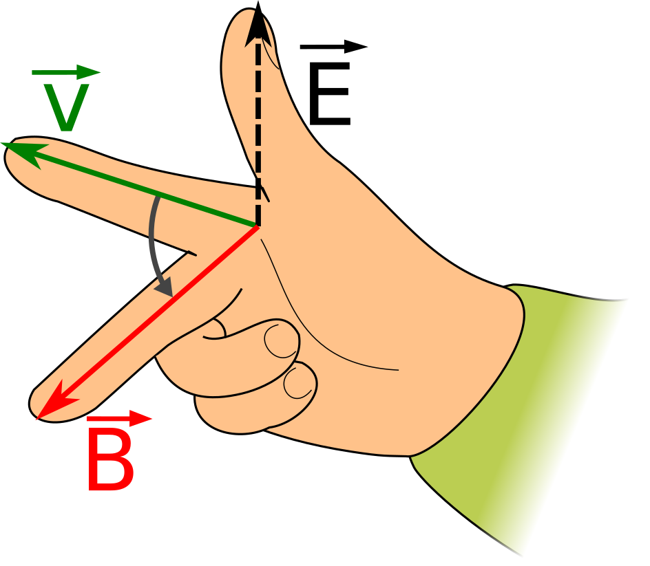
Normally, the value of the electric field is not usually as important as the total voltage, or electromotive force.
The electromotive force is dependent on:
- the electric field; and
- the total length of winding conductor that is parallel to the electric field a.k.a the effective conductor length.
The equation for electromotive force of a moving winding is given below:
\( \mathcal{E} = B l v \sin \theta \)
where \( \mathcal{E} \) is the electromotive force, (V), \( l \) is the effective conductor length (m), v is the magnitude of the velocity of the winding (m.s-1), and \( \theta \) is the angle between the velocity and the magnetic field.
The quantity \( v \sin \theta \) is the component of the velocity at right angles to the magnetic field. This is sometimes referred to as the coil "cutting" magnetic field lines. The faster the coil cuts magnetic field lines, the higher the EMF.
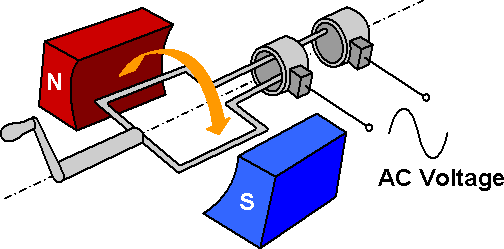
The picture below shows a simple alternator, which is used to generate a voltage by moving a winding in a magnetic field provided by the permanent magnets.
Fleming's Rules
Fleming's Rules are used to determine the direction of the current in a motor or generator winding.
There are two versions: Fleming's Left Hand Rule for Motors, and Fleming's Right Hand Rule for Generators.
The rules are different because the relationship between current and EMF is different for motors and generators.
A motor (or generator) that is rotating in a given direction, with a given magnetic field will always produce the same EMF.
The difference is the following:
- in a generator, the current flow is in the same direction as the the electric field (current is parallel to the electric field); and
- in a motor, the current flow is in the opposite direction to the the electric field (current is anti-parallel to the electric field).
In the right-hand rule for the Lorentz Force, the output (electric field) is on the thumb. In Fleming's Rules, the output (winding current) is on the middle finger.
A version of the Lorentz Force using the middle finger as output is shown below.
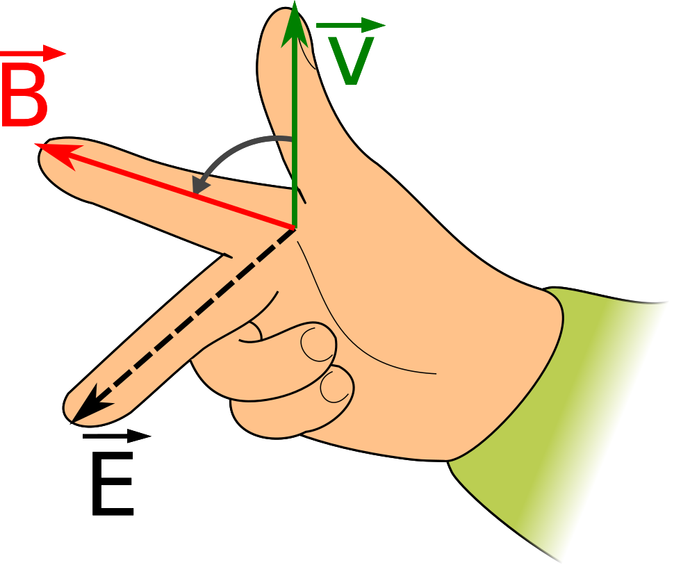
This diagram forms the basis for Fleming's Rules.
Fleming's Right-Hand Rule for Generators
Flemings Right-Hand Rule for Generators is derived from the Lorentz Force in the following way:
- replacing velocity with force (i.e. the force maintaining that velocity in a generator);
- replacing electric field with electric current flowing in the same direction.
Doing these steps produces Fleming's Right-Hand Rule for Generators as pictured below.
\( F \) represents the force exerted on the winding (i.e. the force that makes the winding move), \( B \) represents the magnetic field. and \( i \) represents the direction of induced current flow.
Fleming's Left-Hand Rule for Motors
Flemings Right-Hand Rule for Motors is derived from the Lorentz Force in the following way:
- replacing velocity with force (i.e. the force maintaining that velocity in a generator);
- replacing electric field with electric current flowing in the opposite direction.
Reversing the direction results in a right-hand rule where the current is going in the exact opposite direction to the right middle finger. Luckily, since the left hand is a mirror image of the right hand, the current can be aligned along the middle finger by using the left hand to "mirror" the middle finger.
Doing these steps produces Fleming's Left-Hand Rule for Motors as pictured below.
5. Applications and Examples
Electromagnetism is used in many electrical devices. This chapter goes through some of them.
5.1. Relays and Contactors
Relays and contactors are switches that are activated by electromagnets. They enable a small signal to switch a much larger signal. Relays are generally smaller than contactors and often have two position contacts.
A labelled image of a relay is shown below.
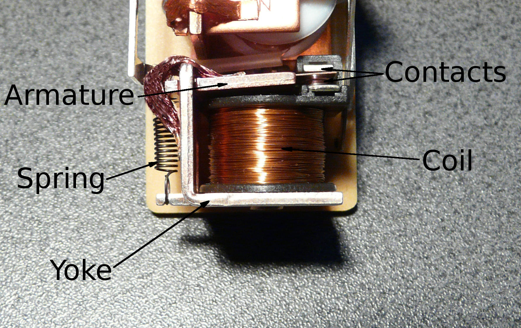
Relays consist of a coil wound on a yoke, and an armature that is moved when a current flows in the relay coil. The movement moves the armature between one or more sets of contacts. When the current stops, the spring on the left pulls the armature to its unenergised position.
No electrical contact is required between the circuit that drives the coil and the switched output. Relays are therefore useful because they provide electrical isolation between the coil and the switched output.
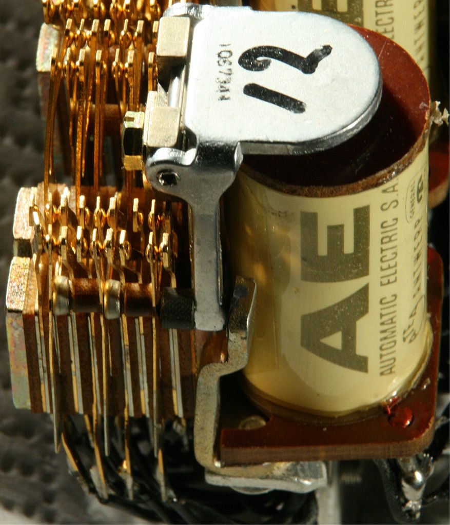
Another example of a relay is shown below. In the relay below, the armature (labelled 12) is pulled down when enough current flows in the coil. The armature is connected mechanically to a spring-loaded contact arm. The movement of the armature will move the contact arm from being in contact with one set of contacts to another. In this way, a relay can be used to switch its outputs. When the current is stopped, the force on the armature stops, and the spring pulls the contact back to its 'off' position.
Contactors
A contactor is similar to a relay except that contactors are designed for higher power circuits. They also have single action contacts that are only designed to switch a load when current is present in the coil. A contactor is shown below.
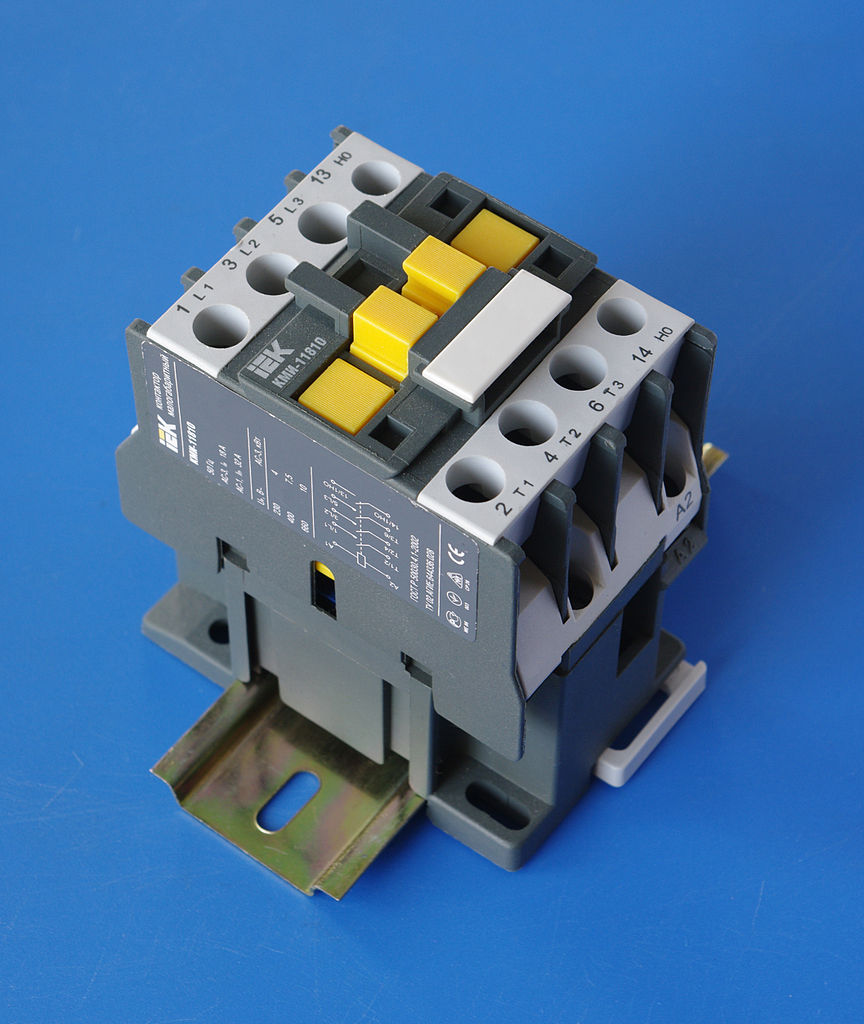
Contactors are designed with auxiliary contacts to signal when the contactor is on or off, and extra devices (e.g. delay timers) can be attached to the armature at top of the contactor (the yellow part).
Relay Contact Configurations
Relays are highly flexible in how their contacts are arranged. Some example arrangements are shown below.
The symbol on the left is the coil. The coil is energised by a control circuit.
An explanation of the contacts follows.
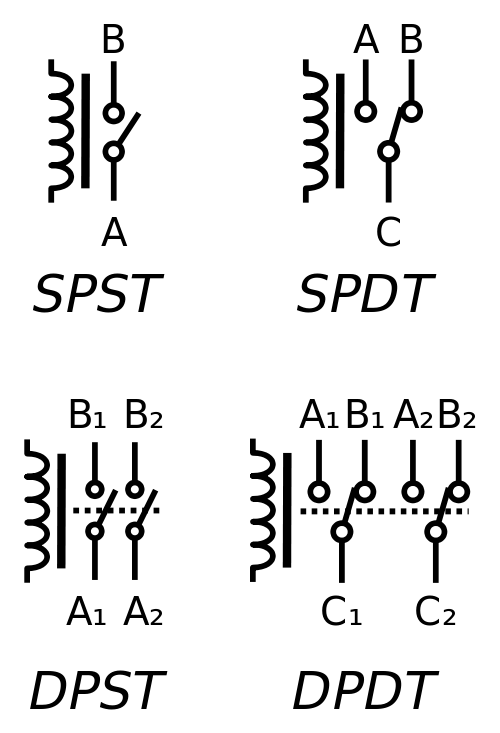
The terminals in the relays above are given letter identifiers. The table below explains how the contacts change.
Poles and Throws
The relays above are defined by poles and throws.
A pole is a set of contacts, denoted by 'P'. SP means 'single pole' (single set of contacts), and DP means 'double pole' (double set of contacts). There is no upper limit on the number of poles. Some relays used in telephone exchanges use 30 poles or more.
A throw is a contact. A single throw pole has a single contact, that is either connected or disconnected when the relay is energised. A double throw pole has two contacts. When the relay is de-energised, the common terminal is connected to one of the throw contacts. When the relay is energised, the common terminal is connected to the other contact.
5.2. Transformers
A transformer uses magnetic fields to transfer energy from one circuit to another.
There are two main types of transformers:
- Isolating transformers, where there are at least two coils. The coils do not need to be electrically connected together. Isolating transformers can have any number of coils.
- Autotransformers, which have one coil only. The output is a connection, or "tap" off the same coil. Autotransformers do not provide electrical isolation between input and output.
Although transformers could theoretically operate off DC, in practice this is not possible because DC would require an unlimited amount of magnetic flux. Therefore, transformers are purely AC devices.
Transformers have a primary winding, and in the case of isolating transformers, one or more secondary windings. Power is transferred from the primary winding to the secondary windings.
The illustration below shows a two-winding transformer. As previously discussed, the two winding are called the primary and secondary windings. The primary winding has \( N_P \) turns, and the secondary winding has \( N_S \) turns.

For an ideal transformer, the following rules hold. A real transformer will not obey these rules, but should be close.
- \( I_P = 0 \) when \( I_S = 0 \) i.e. there is no magnetising current. A real transformer has some magnetising current flowing in the primary at all times.
- \( V_S I_S = V_P I_P \) i.e. no power losses. In a real transformer, \( V_S I_S < V_P I_P \) due to wire and core losses.
- \( V_S = \frac{N_S}{N_P} V_P \) i.e. the secondary voltage is determined only by the turns ratio. In a real transformer, the voltage will be less than this, or extra turns will be added to the secondary to raise the voltage at rated current.
- \( I_S = \frac{N_P}{N_S} I_P \) i.e. the secondary current is determined only by the turns ratio. In a real transformer, the current will be less than this, or extra turns will be added to the primary to raise the current at rated current.
- The primary flux is directly proportional to the primary voltage divided by the primary voltage's frequency and number of turns i.e. \( \Phi \propto \frac{V_P}{N_P f} \), where f is the frequency of the AC supply in hertz.
- The core never saturates.
- All the primary flux links to the secondary (there is no "leakage flux". In practice, there is some leakage flux.
- There is no lower limit on the number of primary turns. In practice, a minimum number of primary turns is required to keep the magnetising current low, and to keep the core from saturating.
- There are no losses from winding resistance. In practice, this must be compensated for in the design.
- There are no core losses. In practice, this must be compensated for in the design, such as by using laminated cores to reduce eddy current losses in the core.
The secondary voltage \( V_S \) is generated by the secondary coils being subject to a changing magnetic field generated by the primary. The changing magnetic field provides the "movement" required to generate an EMF in the secondary coil. In other words, \( V_S = -\mathcal{E} = N_S \frac{\Delta \Phi}{\Delta t} \).
Although the secondary voltage is predicted as being negative, the primary and secondary coils are wound in the opposite directions to each other, so the secondary coil voltage has the same polarity as the primary voltage at all times.
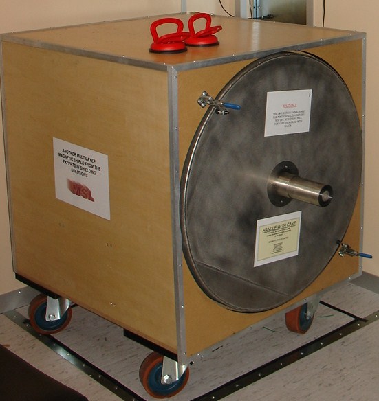
5.3. Magnetic Shielding
Apart from its strength, low price, resistance to fire, and ease of working, steel has two main advantages when making electrical enclosures
- high permeability means it's good for magnetic shielding; and
- being conductive, it blocks electric fields.
Both of these properties help reduce interference from electrical switchgear.
Enclosing equipment that is sensitive to magnetic disturbances (even the Earth's magnetic field can cause problems) within a high permeability enclosure is called magnetic shielding. The idea is to use the high permeability enclosure to divert magnetic fields around the sensitive device.
The picture below shows a box made of mu-metal a special alloy that is designed to magnetically shield a sensitive experiment.
5.4. AC Generator (Alternator)
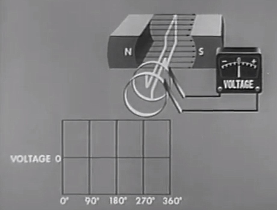
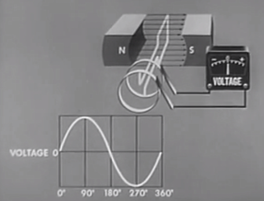
We now turn our attention to an actual example if an AC generator, or alternator. There are a series of five pictures of a single loop alternator at 0°, 90°, 180°, 270° and 360° of rotation. The single loop coil is being turned clockwise.
The path for calculating \( \mathcal{E} \) goes from the front slip ring to the rear slip ring. The parts of the coil that generate an EMF at all the the two parts that are at 90° to the magnetic field lines. The rear part of the coil does not generate any EMF at all, any electric field is always at 90° to the wire.
The simplest form of an AC generator is shown below. The simplest example consists of a single loop of wire, a magnet, slip rings and a load, as shown below.

The basic equation for the voltage from an AC generator is:
\( \mathcal{E}(t) = B l v \sin (\omega t) \)
where \( \mathcal{E}(t) \) is the instantaneous electromotive force (V), \( B \) is the magnetic flux density from the magnet (T), \( l \) is the total length of the wire at 90° to the magnetic field (m), \( v \) is the circular velocity of the coil (m.s-1), \( \omega \) is the angular velocity of the coil (rad.s-1), and \( t \) is time (s). The length \( l \) depends on the number of turns of the generating coil, adding more turns increases the length.
The magnitude of the circular velocity is given by \( v = r \omega \), where \( r \) is the radius of the coil (m). Using \( r \omega \) for the circular velocity gives:
\( \mathcal{E}(t) = B l r \omega \sin (\omega t) \)
This formula shows that the output is proportional to the angular velocity.
Knowing this, these are some ways to increase the peak EMF from the generator:
- Increase \( B \): Use a stronger magnet.
- Increase \( \omega \): Turn the generator faster.
- Increase \( v \) by increasing \( \omega \): Turn the generator faster.
- Increase \( v \) by increasing \( r \): Make the radius of the coils larger.
- Increase \( l \): Make the generator longer.
- Increase \( l \): Put more turns on the generator coil.
Determining "Real-Time" EMF
Determining the behaviour of an alternator can be tricky. The following features of an alternator affect the polarity:
- the direction of rotation as viewed from the slip rings (clockwise or anticlockwise);
- the orientation of the magnetic poles relative to the rotation (N-S or S-N);
- whether the polarity is considered positive at the front slip ring or negative at the front slip ring;
- whether the path of the coil from the negative slip ring to the positive slip ring goes clockwise or anticlockwise relative to the magnetic field at zero degrees of rotation (the winding orientation of the coil).
Changing any one or three of these features will reverse the polarity. Changing two or four of them will not affect the polarity.
We now turn our attention to an actual example. There are a series of five pictures of a single loop alternator at 0°, 90°, 180°, 270° and 360° of rotation. The single loop coil is being turned clockwise.
The path for calculating \( \mathcal{E} \) goes from the front slip ring to the rear slip ring. The parts of the coil that generate an EMF at all the the two parts that are at 90° to the magnetic field lines. The rear part of the coil does not generate any EMF at all, any electric field is always at 90° to the wire.
In terms of the attributes above that affect the polarity, the example alternator has the following attributes.
- the direction of rotation is clockwise as viewed from the slip rings;
- the magnetic poles are oriented N-S;
- the front slip ring is considered the negative terminal, the rear slip ring is considered the positive terminal;
- the coil is wound clockwise relative to the magnetic field, as the correct winding orientation of the coil is found using the left hand, with the thumb pointing in the direction of the magnetic field.
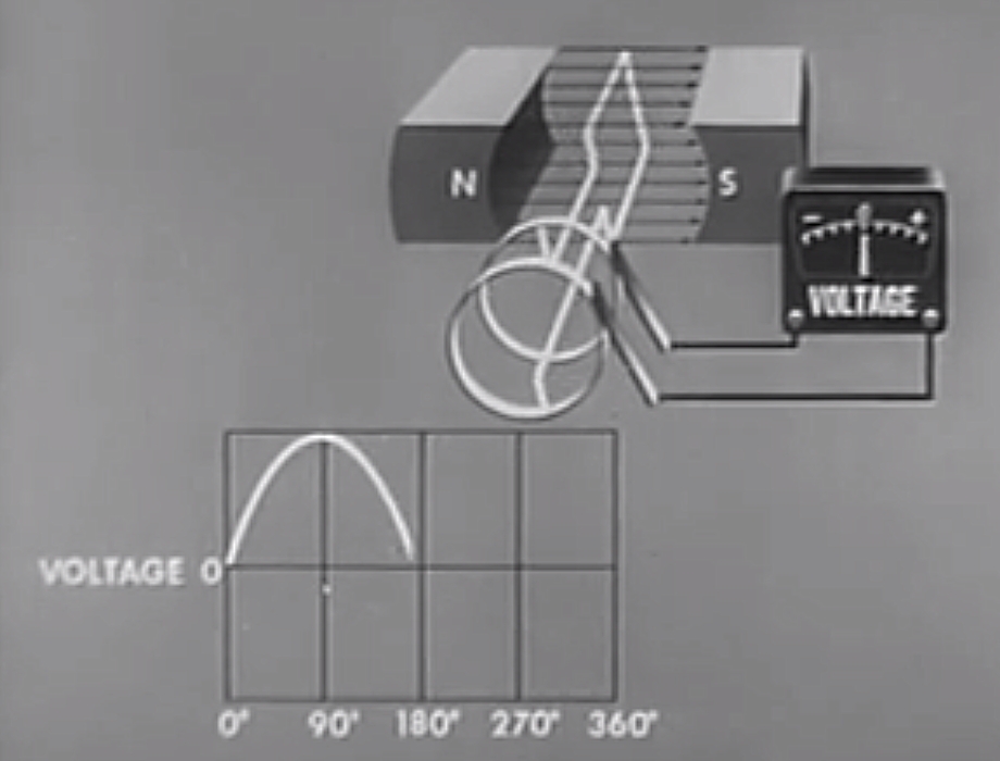
Zero Degrees (\( \theta = 0^{\circ} \))
At zero degrees, the armature is moving to the right (top wire) and left (bottom wire). But the wire is moving parallel to the magnetic field. So \( \theta = 0^{\circ} \), and the EMF is therefore zero too.
90 Degrees (\( \theta = 90^{\circ}\))
At 90 degrees of rotation, the coils are moving at their maximum speed relative to the magnetic field. It can also be said they are "cutting" the maximum number of magnetic field lines.
The EMF is therefore at a maximum, since \( \theta = 90^{\circ} \).
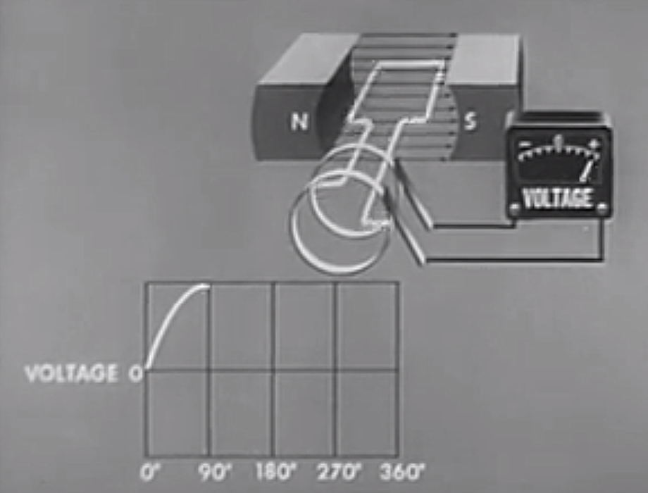
The relative orientations of the magnetic field and velocity will tell us whether the EMF is positive or negative at that instant.
On the right, the velocity is straight down, and the magnetic field is from left to right. Therefore, by \( \vec{E} = \vec{v} \times \vec{B} \), the electric field must be oriented towards the slip rings.
On the left, the velocity is straight up, and the magnetic field is from left to right. Therefore, by \( \vec{E} = \vec{v} \times \vec{B} \), the electric field must be oriented away from the slip rings.
However, because of the orientation of the path of the coil, the electric field in the wire adds up, and therefore the EMF is positive at the slip rings.
180 Degrees (\( \theta = 180^{\circ}\))
The situation at 180 degrees is similar to the situation at zero degrees. The wire is moving parallel to the magnetic field. So \( \theta = 180^{\circ} \), and the EMF is therefore zero too.
270 Degrees (\( \theta = 270^{\circ}\))
At 270 degrees of rotation, the coils are moving at their maximum speed relative to the magnetic field. It can also be said they are "cutting" the maximum number of magnetic field lines. But unlike at \( \theta = 270^{\circ} \), the coil is moving in the opposite direction. The EMF is therefore at a negative maximum, since the movement is in the opposite direction to \( \theta = 90^{\circ} \).

The direction of the induced EMF is actually the same as when \( \theta = 90^{\circ} \). However, the coil is effectively connected to the "opposite" slip rings. This reverses the orientation of the path travelled through the coil to calculate the total EMF. Because the path is in the opposite direction, the EMF is negative.
360 Degrees (\( \theta = 360^{\circ} \))
At 360 degrees, the generator has undergone one full rotation. The position is therefore the same as zero degrees, so the EMF will be the same too. The EMF will therefore be zero again.
RMS and Peak Alternator Output
Given the trickiness of determining the alternator output polarity in real time, it is generally easier to describe the RMS and peak voltages.
| With \( v \) | With \( v = r \omega \) | |
|---|---|---|
| Peak Voltage | \( \mathcal{E}_{\mathrm{pk}} = B l v \) | \( \mathcal{E}_{\mathrm{pk}} = B l r \omega \) |
| RMS Voltage | \( \mathcal{E}_{\mathrm{rms}} = \frac{B l v}{\sqrt{2}} \) | \( \mathcal{E}_{\mathrm{rms}} = \frac{B l r \omega}{\sqrt{2}} \) |
All the symbols have the same meanings as above.
5.5. DC Generator (Dynamo)
The DC generator, or dynamo is broadly similar to the AC generator, except a DC generator has a commutator instead of slip rings. The commutator acts to reverse the polarity of the generated EMF every half cycle. The voltage is converted, or rectified, from AC into pulsating DC. The figure below shows an alternator modified into a dynamo. The commutator, a segmented metal ring, is shown by the arrows.
The commutator is configured to reverse the generated AC at the zero crossings sine waveform, so the equation becomes:
\( \mathcal{E} = B l v |\sin \theta| \)
where all quantities have the same meanings as for the alternator. The \( || \) around the \( \sin \) term mean "absolute value".
We now turn our attention to an actual example. There are a series of five pictures of a single loop dynamo at 0°, 90°, 180°, 270° and 360° of rotation. The single loop coil is being turned clockwise. The upper brush is considered the positive terminal, and the lower brush the negative. The white half of the coil is connected to the white commutator segment, and the black half of the coil is connected to the black commutator segment.
Zero Degrees (\( \theta = 0^{\circ} \))
At zero degrees, the armature is moving to the right (top wire) and left (bottom wire). But the wire is moving parallel to the magnetic field. So \( \theta = 0^{\circ} \), and the EMF is therefore zero too.
The commutator brushes are in contact with both ends of the coil at once. No problems with short circuits will occur, as the generated EMF is zero at this instant.
90 Degrees (\( \theta = 90^{\circ}\))
At 90 degrees of rotation, the coils are moving at their maximum speed relative to the magnetic field. It can also be said they are "cutting" the maximum number of magnetic field lines.
The EMF is therefore at a maximum, since \( \theta = 90^{\circ} \).
The relative orientations of the magnetic field and velocity will tell us whether the EMF is positive or negative at that instant.
On the right, the velocity is straight down, and the magnetic field is from left to right. Therefore, by \( \vec{E} = \vec{v} \times \vec{B} \), the electric field must be oriented towards the commutator.
On the left, the velocity is straight up, and the magnetic field is from left to right. Therefore, by \( \vec{E} = \vec{v} \times \vec{B} \), the electric field must be oriented away from the commutator.
However, because of the orientation of the path of the coil, the electric field in the wire adds up, and therefore the EMF is positive at the at the top brush relative to the bottom brush.
180 Degrees (\( \theta = 180^{\circ}\))
The situation at 180 degrees is similar to the situation at zero degrees. The wire is moving parallel to the magnetic field. So \( \theta = 180^{\circ} \), and the EMF is therefore zero too.
The commutator brushes are in contact with both ends of the coil at once. No problems with short circuits will occur, as the generated EMF is zero at this instant.
270 Degrees (\( \theta = 270^{\circ}\))
At 270 degrees of rotation, the coils are moving at their maximum speed relative to the magnetic field. It can also be said they are "cutting" the maximum number of magnetic field lines. But unlike at \( \theta = 270^{\circ} \), the coil is moving in the opposite direction. The EMF generated by the coil loop is therefore at a negative maximum, since the movement is in the opposite direction to \( \theta = 90^{\circ} \).
Because of the commutator, the induced EMF in the coil loop is at a negative maximum, but the commutator has reversed the connection (notice how the white segment is now on top). The EMF is therefore reversed, resulting in it being at a positive peak again.
360 Degrees (\( \theta = 360^{\circ} \))
At 360 degrees, the generator has undergone one full rotation. The position is therefore the same as zero degrees, so the EMF will be the same too. The EMF will therefore be zero again.
RMS, Peak and Average Dynamo Output
Given the trickiness of determining the alternator output polarity in real time, it is generally easier to describe the RMS and peak voltages.
| With \( v \) | With \( v = r \omega \) | |
|---|---|---|
| Peak Voltage | \( \mathcal{E}_{\mathrm{pk}} = B l v \) | \( \mathcal{E}_{\mathrm{pk}} = B l r \omega \) |
| RMS Voltage | \( \mathcal{E}_{\mathrm{rms}} = \frac{B l v}{\sqrt{2}} \) | \( \mathcal{E}_{\mathrm{rms}} = \frac{B l r \omega}{\sqrt{2}} \) |
| Average Voltage | \( \mathcal{E}_{\mathrm{avg}} = \frac{2 B l v}{\pi} \) | \( \mathcal{E}_{\mathrm{avg}} = \frac{2 B l r \omega}{\pi} \) |
6. AC Electricity
This chapter deals with AC electricity, including the sine wave form, RMS and average calculations.
6.1. Sine Waveforms
We have already seen that the output from an AC generator uses the \( \sin \) function.
There are two functions that form a sine wave:
- sine, denoted \( \sin \);
- cosine, denoted \( \cos \).
Sine and Cosine Definitions
The sine and cosine functions are orthogonal in the sense that any sinusoid or sinusoidal wave can be expressed as the sum of a sine wave and a cosine wave.
The sine and cosine waveforms are shown below for a single cycle.
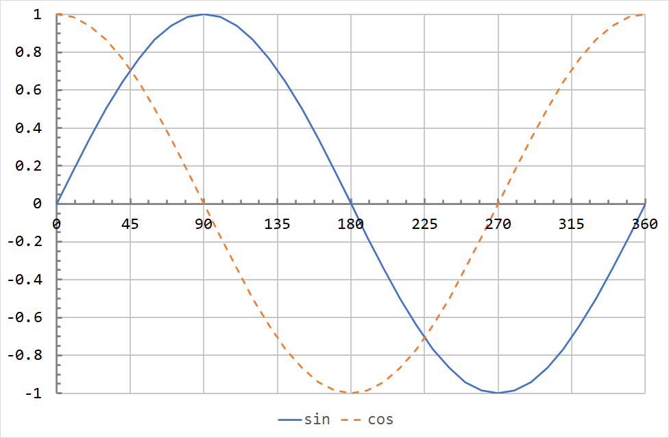
As can be seen, the sine and cosine waves have identical shapes. Sinusoids have a property called phase, which determines the horizontal offset from a reference wave.
For sine waves and cosine waves, some useful relationships are shown below:
- \( \cos(-\theta) = \cos(\theta) \): cosine is an even function, in the sense that it has symmetry around \( \theta = 0 \).
- \( \sin(-\theta) = -\sin(\theta) \): sine is an odd function, in the sense that it has anti-symmetry around \( \theta = 0 \).
- \( \cos \theta = \sin(90^{\circ} - \theta) \): the "standard" cosine-sine conversion.
- \( \sin \theta = \cos(90^{\circ} - \theta) \): the "standard" sine-cosine conversion.
- \( \cos \theta = -\sin(\theta - 90^{\circ}) \): similar to #3, except \( \theta \) is made positive.
- \( \sin \theta = \cos(\theta - 90^{\circ}) \): similar to #4, except \( \theta \) is made positive.
- \( \sin \theta = \sin(\theta + n \cdot 360^{\circ}) \): sinusoids are periodic, with a period of 360°. This also applies to cosine waves.
- \( \sin(\theta + \phi) = \sin\theta \sin \phi + \cos \theta \cos \phi \): every sine wave with a phase shift can be decomposed into the sum of a sine wave and a cosine wave.
- \( \cos(\theta + \phi) = \cos\theta \cos \phi - \sin \theta \sin \phi \): every cosine wave with a phase shift can be decomposed into the sum of a cosine wave and a sine wave.
A parametric plot of sine and cosine shown below. The x-axis is horizontal, and the y-axis is vertical. The parametric plot coordinates are \( (x, y) = (\cos\theta, \sin\theta) \). In other words, it is the graph above, but with the functions plotted against each other, rather than angle. The plot begins at (1, 0) (the far right) and proceeds in a circle anti-clockwise.
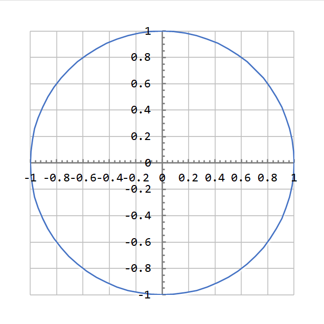
The parametric plot implies one more important identity:
- \( \sin^2 \theta + \cos^2 \theta = 1 \).
Using Radians
In circuit analysis, it is more common to work with angles in radians. Using radians makes the expression of a sine wave as a function of frequency very simple.
The rules above apply as below for radians:
- \( \cos(-\theta) = \cos(\theta) \): no difference from above.
- \( \sin(-\theta) = -\sin(\theta) \): no difference from above.
- \( \cos \theta = \sin(\frac{\pi}{2} - \theta) \): the "standard" cosine-sine conversion.
- \( \sin \theta = \cos(\frac{\pi}{2} - \theta) \): the "standard" sine-cosine conversion.
- \( \cos \theta = -\sin(\theta - \frac{\pi}{2}) \): similar to #3, except \( \theta \) is made positive.
- \( \sin \theta = \cos(\theta - \frac{\pi}{2}) \): similar to #4, except \( \theta \) is made positive.
- \( \sin \theta = \sin(\theta + 2 \pi n) \): sinusoids are periodic, with a period of \( 2 \pi \). This also applies to cosine waves.
- \( \sin(\theta + \phi) = \sin\theta \sin \phi + \cos \theta \cos \phi \): no difference from above.
- \( \cos(\theta + \phi) = \cos\theta \cos \phi - \sin \theta \sin \phi \): no difference from above.
For convenience, a phase shift may be written in degrees anyway e.g. \( \cos (\theta + 45^{\circ}) \). You must remember to convert the phase shift to radians before doing any calculations.
Sinusoids in Circuit Analysis
Sinusoids in circuit analysis are usually expressed in the following forms:
- \( u(t) = A \sin (2 \pi f t + \phi) \); and
- \( u(t) = A \cos (2 \pi f t + \phi) \)
where:
- \( A \) is the amplitude, or peak of the sinusoid;
- \( f \) is the frequency (Hz);
- \( t \) is time (s);
- and \( \phi \) is the phase shift.
The sine and cosines in the formula above use radians as the angle unit. There are \( 2 \pi \) (≈ 6.283) radians in a full revolution, or 1 rad ≈ 57.296°, or 1° ≈ 0.01745 rad.
The factor \( 2 \pi f \) may be factored into angular frequency \( \omega \) (small Greek letter omega). The unit of \( \omega \) is rad.s-1. Using \( \omega \) changes the expressions to:
- \( u(t) = A \sin (\omega t + \phi) \); and
- \( u(t) = A \cos (\omega t + \phi) \)
The waveforms may also be expressed using the period or cycle length of the wave. The period is denoted \( T \) and is the time required for one cycle of the wave. The unit of the period is s.
The relationship between the period and frequency is:
\( f = \frac{1}{T} \)
where \( f \) is the frequency (Hz), and \( T \) is the period (s).
6.2. RMS (Root Mean Square) and Average Derivations
The RMS (root-mean-square) value of an AC waveform is used to relate the effect of AC voltages and currents to an equivalent DC voltage and current. Most AC meters are also calibrated to read RMS voltages and currents!
Consider the circuit below. The lightbulbs are identical, and the AC and DC circuits have been adjusted so that the lightbulbs are of identical brightness. How do we compare the DC current to the AC current?
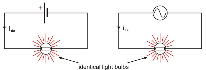
We already know equations like \( P = \frac{V^2}{R} \), \( P = I^2 R \), and \( P = V I \) in DC circuits. But in an AC or pulsating DC system, the voltage is changing all the time, so how can we describe these values?
The RMS (root mean square) value comes to the rescue.
The RMS of a quantity is denoted by a capital letter (e.g. \( V \) for a voltage), and has the following formula:
\( V = \sqrt{\langle v^2 \rangle} \)
where \( V \) is the RMS value of the waveform over a cycle, \( v \) is the instantaneous value of the waveform, and the angle brackets \( \langle \rangle \) mean the average value over an entire cycle.
Different waveforms have different RMS values, we will concentrate on sinusoidal waves and DC in this course.
Here are some some properties of the RMS:
- The constant property. \(\sqrt{\langle A^2 \rangle} = |A| \): The RMS of a constant value \( A \) is the absolute value absolute value of \( A \).
- The amplitude scaling property. \(\sqrt{\langle A^2 v^2 \rangle} = |A| \cdot \sqrt{\langle v^2 \rangle}\): Scaling the waveform by a constant amplitude \( A \) is equal to multiplying the unscaled RMS quantity by the absolute value of \( A \).
- The time scaling property. \(\sqrt{\langle (v(c_1 t))^2 \rangle} = \sqrt{\langle (v(c_2 t))^2 \rangle}\): As long as the RMS is done over a complete cycle, the RMS does not depend on the frequency of the waveform.
- The time shifting property. \(\sqrt{\langle (v(t + T))^2 \rangle} = \sqrt{\langle v^2 \rangle}\): The RMS value is calculated over a complete cycle, so shifting the waveform does by cycle length \( T \) not affect the RMS value.
RMS of DC
In DC circuits, the voltages and currents are constant all the time. Although the cycle length of DC is theoretically infinite, we can in practice take any time value.
Due to the constant property, the RMS value of a DC voltage or current is just the absolute value.
- A DC current \( I_{\mathrm{dc}} \) = 5 A will have an RMS value of 5 A.
- A DC current \( I_{\mathrm{dc}} \) = -5 A (the current might be negative due to the definition of the current flow path) will have an RMS value of 5 A.
- A DC voltage \( V_{\mathrm{dc}} \) = 10 V will have an RMS value of 10 V.
- A DC voltage \( V_{\mathrm{dc}} \) = -10 V (the voltage might be negative due to the definition positive and negative for measurement) will have an RMS value of 10 V.
RMS of Sinusoids
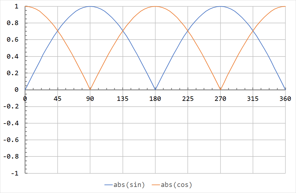
The RMS is based on the average value of the square of a waveform over a cycle. The squared sine and cosine waveforms are shown below for a full 360° cycle.
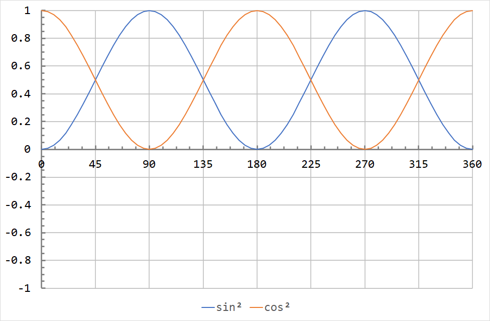
It appears that both waves are symmetric about 0.5. This is true, the mean squared value (MS) for any sinusoid with an amplitude of 1 is 0.5. The RMS is the square root of this value, so the RMS of the sine and cosine waves above is \( \sqrt{0.5} = \sqrt{\frac{1}{2}} = \frac{1}{\sqrt{2}} \approx 0.7071 \).
Note that the sine and cosine waves have identical mean square behaviour. The phase of a sinusoid does not affect the RMS value.
In other words (we are using \( \sin \) here, but it applies equally to any sinusoid):
- \( \langle \sin^2 \theta \rangle = \frac{1}{2} \) for any sinusoid with an amplitude of 1.
- \( \sqrt{\langle \sin^2 \theta \rangle} = \frac{1}{\sqrt{2}} \) for any sinusoid with an amplitude of 1.
We can use the scaling property to get the RMS value of a sinusoid with an amplitude other than one. Consider a sinusoid with an amplitude \( A \). By the scaling property the RMS value is:
\( \sqrt{\langle (A \sin \theta)^2 \rangle} = \frac{A}{\sqrt{2}} \).
If we assume that \( A \) is always positive, we can drop the absolute value signs.
Comparing AC RMS to DC
Consider the AC and DC circuits above. What amplitude does the AC current \( i_{\mathrm{ac}} \) need to have to have the same effect on the load as the DC current \( I_{\mathrm{dc}} \)?
AC Current RMS
As a starting point, we can compute the RMS AC current \( I_{\mathrm{ac}} \).
We will write the AC current as:
\( i_{\mathrm{ac}} = I_{\mathrm{pk}} \sin (2 \pi f t ) \)
where \( i_{\mathrm{ac}} \) is the instantaneous AC current (A), \( I_{\mathrm{pk}} \) is theamplitudeorpeakof the AC current waveform (A), \( f \) is the frequency (Hz), and \( t \) is time (s). We will assume that \( I_{\mathrm{pk}} \) is positive.
Using the properties of the RMS, we can get that \( I_{\mathrm{ac}} = \frac{I_{\mathrm{pk}}}{\sqrt{2}} \).
- \( I_{\mathrm{ac}} = \sqrt{i_{\mathrm{ac}}^2} \) (RMS formula)
- \( I_{\mathrm{ac}} = \sqrt{I_{\mathrm{pk}}^2 \sin^2 (2 \pi f t ) }\) (waveform substitution)
- \( I_{\mathrm{ac}} = I_{\mathrm{pk}} \sqrt{\sin^2 (2 \pi f t ) }\) (amplitude scaling property)
- \( I_{\mathrm{ac}} = I_{\mathrm{pk}} \sqrt{\sin^2 \theta }\) (time scaling property)
- \( I_{\mathrm{ac}} = I_{\mathrm{pk}} \cdot \frac{1}{\sqrt{2}} \) (waveform RMS substitution)
In other words, the RMS AC current\( I_{\mathrm{ac}} \) is \( \frac{1}{\sqrt{2}} \) times the peak current \( I_{\mathrm{pk}} \). We will keep that in mind for the the next section involving the power.
Average AC Power
The instantaneous AC power is given by:
\( p_{\mathrm{ac}} = R i_{\mathrm{ac}}^2 \)
where \( R \) is the load resistance, and \( i_{\mathrm{ac}} \) is the instantaneousAC current.
The instantaneous power can therefore be written:
\( p_{\mathrm{ac}} = R \cdot I_{\mathrm{pk}}^2 \sin^2 (2 \pi f t ) \)
In order to compare the response to the DC response, we are interested in the average power \( P_{\mathrm{ac}} \) over a whole cycle.
\( P_{\mathrm{ac}} = \langle p_{\mathrm{ac}} \rangle \)
\( P_{\mathrm{ac}} = \langle R \cdot I_{\mathrm{pk}}^2 \sin^2 (2 \pi f t ) \rangle\)
\( P_{\mathrm{ac}} = R I_{\mathrm{pk}}^2 \cdot \langle \sin^2 (2 \pi f t ) \rangle \)
\( P_{\mathrm{ac}} = R \cdot \frac{I_{\mathrm{pk}}^2}{2} \)
But \( I_{\mathrm{ac}} = I_{\mathrm{pk}} \cdot \frac{1}{\sqrt{2}} \), so we can write the average ac power as
\( P_{\mathrm{ac}} = R \cdot I_{\mathrm{ac}}^2 \)
In other words:
- the average power is the resistance multiplied by the square of the RMS AC current i.e. \( P_{\mathrm{ac}} = I_{\mathrm{ac}}^2 R \).
- the average power will be the same if the RMS AC current is the same as the DC current i.e. \( I_{\mathrm{ac}} = I_{\mathrm{dc}} \).
Similar calculations apply to the voltage.
Average of Sinusoids
On the face of it, the average value is a sinusoid is zero. The average in this context refers tho the average of the absolute value of the sinusoid, or the rectified sinusoidal waveform.
The average is what a DC voltmeter would read if connected to rectified AC. It is also used by cheaper multimeters to give an AC measurement.
The rectified (or absolute value) AC sine and cosine waves are shown below. Since they are (almost always) above zero the entire cycle, their average will be non-zero.
The exact mathematics are beyond the scope of this course, but the average of a sinusoid is \( \frac{2}{\pi} = 0.6366 \) times its peak value. If the y-axis represented volts, and a DC voltmeter were connected to the waveform above, it would read about 0.6366 V.
The average is also important because many cheaper multimeters are not "True RMS". Rather than calculating the RMS in real time like above, they measure the average waveform by rectifying and filtering, then by a constant to turn it into an RMS value.
\( U_{\mathrm{ac}} = \frac{U_{\mathrm{ac}}}{U_{\mathrm{pk}}} \cdot \frac{U_{\mathrm{pk}}}{U_{\mathrm{avg}}}\cdot U_{\mathrm{avg}} = \frac{1}{\sqrt{2}} \cdot \frac{\pi}{2} \cdot U_{\mathrm{avg}} = \frac{\pi}{2 \sqrt{2}} U_{\mathrm{avg}} \approx 1.111 U_{\mathrm{avg}} \)
This approximation works only if the waveform being measured is close to sinusoidal. In practice, voltages (except from devices like light dimmers) are mostly close to being sinusoidal. Currents in AC circuits tend not to be as sinusoidal due to transformers and electronic loads.
6.3. RMS, Peak, Peak-to-Peak and Average Summary
RMS, Peak, and Peak-to-Peak Conversions
The figure shows a summary of the different peak and RMS measurements for a given AC voltage waveform.
The waveform equation is:
\( y = V_{\mathrm{pk}} \sin \theta \)

The table below shows the ratios for conversion between peak, RMS, peak-to-peak and such. For example, to convert an RMS value to a peak value, look up RMS in the left column, then look up Peak in the top row, and look at the value where the RMS row and the Peak column intersect.
| RMS | Average | Peak | Peak-to-Peak | |
|---|---|---|---|---|
| RMS | 1 | \( \frac{2 \sqrt{2}}{\pi} \) (0.9003) | \( \sqrt{2} \) (1.414) | \( 2 \sqrt{2} \) (2.828) |
| Average | \( \frac{\pi}{2 \sqrt{2}} \) (1.111) | 1 | \( \frac{\pi}{2} \) (1.571) | \( \pi \) (3.142) |
| Peak | \( \frac{1}{\sqrt{2}} \) (0.7071) | \( \frac{2}{\pi} \) (0.6366) |
1 | 2 |
| Peak-to-Peak | \( \frac{1}{2 \sqrt{2}} \) (0.3536) | \( \frac{1}{\pi} \) (0.3183) | 0.5 | 1 |
The table below shows the formulas for converting between period, frequency and angular frequency. For example, to convert an frequency to angular frequency, look up Frequency in the left column, then look up Angular Frequency in the top row, and look at the formula where the Frequency row and the Angular Frequency column intersect.
| Frequency \( f \) | Period \( T \) | Angular Frequency \( \omega \) | |
|---|---|---|---|
| Frequency \( f \) | 1 | \( \frac{1}{f} \) | \( 2 \pi f \) |
| Period \( T \) | \( \frac{1}{T} \) |
1 | \( \frac{2 \pi}{T} \) |
| Angular Frequency \( \omega \) | \( \frac{\omega}{2 \pi} \) | \( \frac{2 \pi}{\omega} \) |
1 |
The mains supply in New Zealand is 230 V RMS. The values of RMS voltage, peak voltage, peak-to-peak voltage, frequency, period and angular frequency are as shown below. The values use the conversion factors and formulas provided in the tabels above.
| RMS | Average | Peak | Peak-to-Peak | |
|---|---|---|---|---|
| RMS | 230 V | 207.1 V | 325.3 V | 650.5 V |
| Frequency \( f \) | Period \( T \) | Angular Frequency \( \omega \) | |
|---|---|---|---|
| Frequency \( f \) | 50 Hz | 0.02 s | 314.2 rad.s-1 |
The graph below is a plot of the mains voltage over a single cycle. The cycle length is 0.02 s, since the mains has a frequency of 50 Hz in New Zealand.
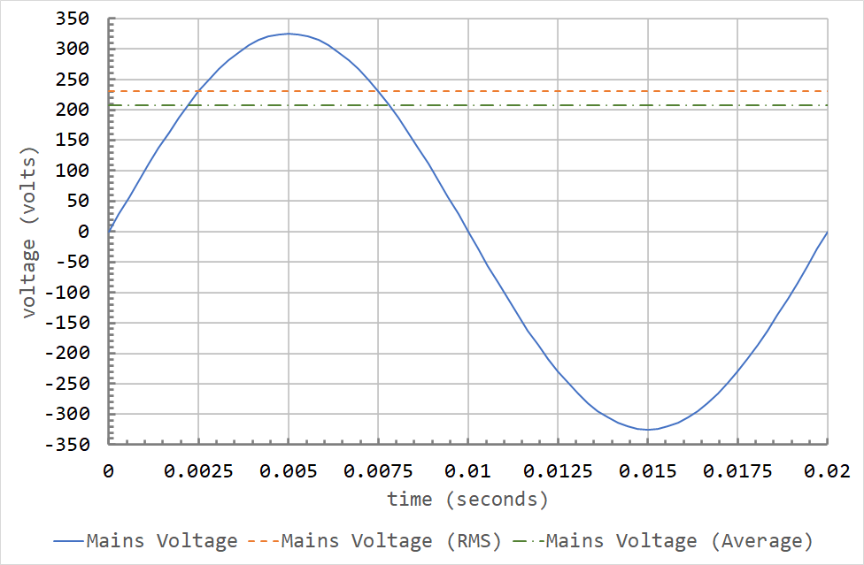
It is no coincidence that the RMS value crosses the sine wave at 0.0025 and 0.0075 seconds. These correspond to \( \theta = 45^{\circ} \) and \( \theta = 135^{\circ} \). The sine of both \( 45^{\circ} \) and \( 135^{\circ} \) is 0.7071, which is \( \frac{1}{\sqrt{2}} \).