Electromagnetism Resource
4. Electromagnetic Effects
4.4. Electromagnetic Induction in Stationary Coils and Transformers (Faraday's Law)
Faraday's Law of Induction relates an electromotive force generated in a length of wire to the rate of change of the magnetic flux passing through the coil with respect to time.
The changing magnetic flux generates a curled electric field i.e. an electric field that goes in loops. Using a wire (or a coil) captures this looped electric field, generating an EMF.
Faraday's Law of Induction is:
\( \mathcal{E} = -N \frac{\Delta \Phi}{\Delta t} \)
where \( \mathcal{E} \) is the electromotive force (V), N is the number of turns of the coil (dimensionless), and \( \Phi \) is the magnetic flux passing through the coil (Wb). The quantity \( \frac{\Delta \Phi}{\Delta t} \) represents the rate of change of the magnetic flux with respect to time (Wb.s-1 or V).
The EMF is negative because it always tries to oppose the change in magnetic field.
The picture below shows an example of this phenomenon. The magnet is moving, subjecting the coil to a changing magnetic flux. This changing magnetic flux causes an EMF to be induced in the coil, making the needle on the galvanometer move.
The EMF can also be related to the magnetic flux density, if the area of the coil is known. This form is shown below.
\( \mathcal{E} = -N A \frac{\Delta B}{\Delta t} \)
where \( \mathcal{E} \) is the electromotive force (V), N is the number of turns of the coil, \( A \) is the enclosed area of the coil, and \( B \) is the magnetic flux density (T). The quantity \( \frac{\Delta B}{\Delta t} \) represents the rate of change of the magnetic flux density with respect to time (T.s-1).
Transformers
Transformers make use of Faraday's Law of Induction. An illustration of a transformer is shown below.
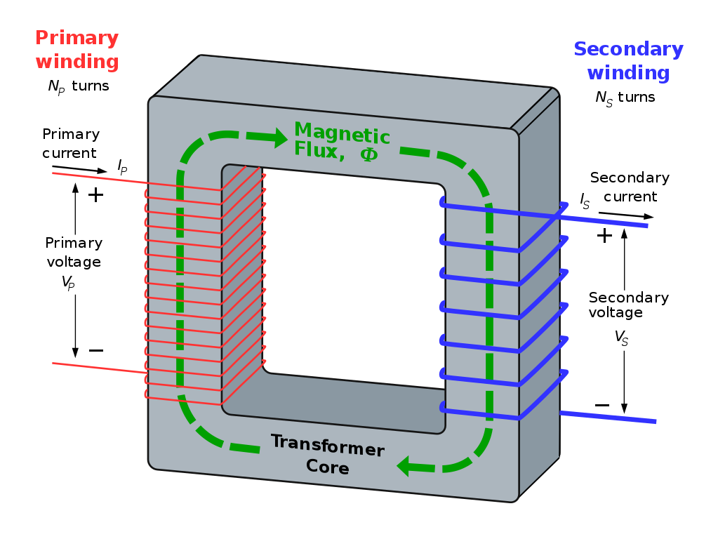
The current flowing through the primary winding generates a magnetic flux \( \Phi \). The magnetic flux travels through the high-permeability core, and intercepts the secondary winding.
If the magnetic flux is changing, an EMF (the secondary voltage) will be generated in the secondary coil.
The induced EMF in the secondary coil can be used to power a load.
The advantages of transformers are the following:
- they can change voltages and currents i.e. they can step-up or step-down voltages and currents;
- there is no electrical contact required between the primary and secondary i.e. transformers can provide electrical isolation.
The ability to electrically isolate the primary and secondary is a major safety benefit.
The secondary voltage can be changed by varying the number of turns on the secondary winding.
Transformers are not DC devices. Operating a transformer at DC would require two things:
- unlimited magnetic flux; and
- windings without any resistance.
While it is possible to use super-conductors with zero resistance for the windings, it is not possible to have unlimited magnetic flux. In practice, transformers can only be used with alternating current.
Calculating Transformer Voltages and Currents
Assuming the resistance of a transformer winding is small (so that any primary resistance causes a small voltage drop due to primary current \( I_{\mathrm{p}} \), the rate of change of flux on the primary coil is the same as the primary voltage \( V_\mathrm{p} \).
\( V_{\mathrm{p}} = -N_{\mathrm{p}} \frac{\Delta \Phi_{\mathrm{p}}}{\Delta t} \)
On the secondary side, a similar situation applies.
\( V_{\mathrm{s}} = -N_{\mathrm{s}} \frac{\Delta \Phi_{\mathrm{s}}}{\Delta t} \)
Note that the secondary voltage is dependent on \( \Phi_{\mathrm{s}} \), the magnetic flux passing through the secondary. In a "good" transformer, the secondary flux will be nearly the same as the primary flux, so \( \Phi_{\mathrm{s}} \) can be replaced with \( \Phi_{\mathrm{p}} \).
\( V_{\mathrm{s}} = -N_{\mathrm{s}} \frac{\Delta \Phi_{\mathrm{p}}}{\Delta t} \)
This allows us to derive a relationship between the primary and secondary voltages.
\( \frac{V_{\mathrm{p}}}{V_{\mathrm{s}}} = \frac{-N_{\mathrm{p}} \frac{\Delta \Phi_{\mathrm{p}}}{\Delta t}}{-N_{\mathrm{s}} \frac{\Delta \Phi_{\mathrm{p}}}{\Delta t}} = \frac{N_{\mathrm{p}}}{N_{\mathrm{s}}} \)
\( V_{\mathrm{s}} = \frac{N_{\mathrm{s}}}{N_{\mathrm{p}}} V_{\mathrm{p}} \)
The primary and secondary currents are calculated by observing that the magnetising forces from the primary and secondary windings must balance.\( H_{\mathrm{p}} = k N_{\mathrm{p}} I_{\mathrm{p}} \)
\( H_{\mathrm{s}} = k N_{\mathrm{s}} I_{\mathrm{s}} \)
The value \( k \) depends on the exact details of the transformer construction, but it is assumed that \( k \) is the same for both primary and secondary windings.
\( \frac{H_{\mathrm{p}}}{H_{\mathrm{s}}} = 1 = \frac{k N_{\mathrm{p}} I_{\mathrm{p}}}{k N_{\mathrm{s}} I_{\mathrm{s}}} = \frac{N_{\mathrm{p}} I_{\mathrm{p}}}{N_{\mathrm{s}} I_{\mathrm{s}}} \)
The equation for the secondary current is shown below. Note that the ratio for the current is the inverse of the ratio for the voltage. This is because transformers cannot add power, at best they can only conserve it. Therefore \( V_{\mathrm{p}} I_{\mathrm{p}} \geq V_{\mathrm{s}} I_{\mathrm{s}} \). This condition is achieved if the voltage ratio is \( \frac{N_{\mathrm{s}}}{N_{\mathrm{p}}} \) and the current ratio is \( \frac{N_{\mathrm{p}}}{N_{\mathrm{s}}} \).
The equation for the secondary current in terms of the primary current is shown below.
\( I_{\mathrm{s}} = \frac{N_{\mathrm{p}}}{N_{\mathrm{s}}} I_{\mathrm{p}} \)
NOTE: These equations only apply to an ideal transformer. A real transformer will have a current flow in the primary winding even when there is no current in the secondary, for example. But these equations form the basis for evaluating the performance of transformers.