Electromagnetism Resource
6. AC Electricity
6.2. RMS (Root Mean Square) and Average Derivations
The RMS (root-mean-square) value of an AC waveform is used to relate the effect of AC voltages and currents to an equivalent DC voltage and current. Most AC meters are also calibrated to read RMS voltages and currents!
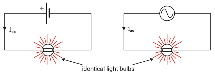
Consider the circuit below. The lightbulbs are identical, and the AC and DC circuits have been adjusted so that the lightbulbs are of identical brightness. How do we compare the DC current to the AC current?
We already know equations like \( P = \frac{V^2}{R} \), \( P = I^2 R \), and \( P = V I \) in DC circuits. But in an AC or pulsating DC system, the voltage is changing all the time, so how can we describe these values?
The RMS (root mean square) value comes to the rescue.
The RMS of a quantity is denoted by a capital letter (e.g. \( V \) for a voltage), and has the following formula:
\( V = \sqrt{\langle v^2 \rangle} \)
where \( V \) is the RMS value of the waveform over a cycle, \( v \) is the instantaneous value of the waveform, and the angle brackets \( \langle \rangle \) mean the average value over an entire cycle.
Different waveforms have different RMS values, we will concentrate on sinusoidal waves and DC in this course.
Here are some some properties of the RMS:
- The constant property. \(\sqrt{\langle A^2 \rangle} = |A| \): The RMS of a constant value \( A \) is the absolute value absolute value of \( A \).
- The amplitude scaling property. \(\sqrt{\langle A^2 v^2 \rangle} = |A| \cdot \sqrt{\langle v^2 \rangle}\): Scaling the waveform by a constant amplitude \( A \) is equal to multiplying the unscaled RMS quantity by the absolute value of \( A \).
- The time scaling property. \(\sqrt{\langle (v(c_1 t))^2 \rangle} = \sqrt{\langle (v(c_2 t))^2 \rangle}\): As long as the RMS is done over a complete cycle, the RMS does not depend on the frequency of the waveform.
- The time shifting property. \(\sqrt{\langle (v(t + T))^2 \rangle} = \sqrt{\langle v^2 \rangle}\): The RMS value is calculated over a complete cycle, so shifting the waveform does by cycle length \( T \) not affect the RMS value.
RMS of DC
In DC circuits, the voltages and currents are constant all the time. Although the cycle length of DC is theoretically infinite, we can in practice take any time value.
Due to the constant property, the RMS value of a DC voltage or current is just the absolute value.
- A DC current \( I_{\mathrm{dc}} \) = 5 A will have an RMS value of 5 A.
- A DC current \( I_{\mathrm{dc}} \) = -5 A (the current might be negative due to the definition of the current flow path) will have an RMS value of 5 A.
- A DC voltage \( V_{\mathrm{dc}} \) = 10 V will have an RMS value of 10 V.
- A DC voltage \( V_{\mathrm{dc}} \) = -10 V (the voltage might be negative due to the definition positive and negative for measurement) will have an RMS value of 10 V.
RMS of Sinusoids
The RMS is based on the average value of the square of a waveform over a cycle. The squared sine and cosine waveforms are shown below for a full 360° cycle.
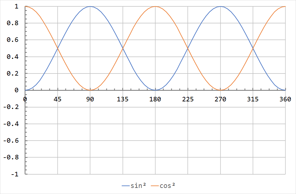
It appears that both waves are symmetric about 0.5. This is true, the mean squared value (MS) for any sinusoid with an amplitude of 1 is 0.5. The RMS is the square root of this value, so the RMS of the sine and cosine waves above is \( \sqrt{0.5} = \sqrt{\frac{1}{2}} = \frac{1}{\sqrt{2}} \approx 0.7071 \).
Note that the sine and cosine waves have identical mean square behaviour. The phase of a sinusoid does not affect the RMS value.
In other words (we are using \( \sin \) here, but it applies equally to any sinusoid):
- \( \langle \sin^2 \theta \rangle = \frac{1}{2} \) for any sinusoid with an amplitude of 1.
- \( \sqrt{\langle \sin^2 \theta \rangle} = \frac{1}{\sqrt{2}} \) for any sinusoid with an amplitude of 1.
We can use the scaling property to get the RMS value of a sinusoid with an amplitude other than one. Consider a sinusoid with an amplitude \( A \). By the scaling property the RMS value is:
\( \sqrt{\langle (A \sin \theta)^2 \rangle} = \frac{A}{\sqrt{2}} \).
If we assume that \( A \) is always positive, we can drop the absolute value signs.
Comparing AC RMS to DC
Consider the AC and DC circuits above. What amplitude does the AC current \( i_{\mathrm{ac}} \) need to have to have the same effect on the load as the DC current \( I_{\mathrm{dc}} \)?
AC Current RMS
As a starting point, we can compute the RMS AC current \( I_{\mathrm{ac}} \).
We will write the AC current as:
\( i_{\mathrm{ac}} = I_{\mathrm{pk}} \sin (2 \pi f t ) \)
where \( i_{\mathrm{ac}} \) is the instantaneous AC current (A), \( I_{\mathrm{pk}} \) is theamplitudeorpeakof the AC current waveform (A), \( f \) is the frequency (Hz), and \( t \) is time (s). We will assume that \( I_{\mathrm{pk}} \) is positive.
Using the properties of the RMS, we can get that \( I_{\mathrm{ac}} = \frac{I_{\mathrm{pk}}}{\sqrt{2}} \).
- \( I_{\mathrm{ac}} = \sqrt{i_{\mathrm{ac}}^2} \) (RMS formula)
- \( I_{\mathrm{ac}} = \sqrt{I_{\mathrm{pk}}^2 \sin^2 (2 \pi f t ) }\) (waveform substitution)
- \( I_{\mathrm{ac}} = I_{\mathrm{pk}} \sqrt{\sin^2 (2 \pi f t ) }\) (amplitude scaling property)
- \( I_{\mathrm{ac}} = I_{\mathrm{pk}} \sqrt{\sin^2 \theta }\) (time scaling property)
- \( I_{\mathrm{ac}} = I_{\mathrm{pk}} \cdot \frac{1}{\sqrt{2}} \) (waveform RMS substitution)
In other words, the RMS AC current\( I_{\mathrm{ac}} \) is \( \frac{1}{\sqrt{2}} \) times the peak current \( I_{\mathrm{pk}} \). We will keep that in mind for the the next section involving the power.
Average AC Power
The instantaneous AC power is given by:
\( p_{\mathrm{ac}} = R i_{\mathrm{ac}}^2 \)
where \( R \) is the load resistance, and \( i_{\mathrm{ac}} \) is the instantaneousAC current.
The instantaneous power can therefore be written:
\( p_{\mathrm{ac}} = R \cdot I_{\mathrm{pk}}^2 \sin^2 (2 \pi f t ) \)
In order to compare the response to the DC response, we are interested in the average power \( P_{\mathrm{ac}} \) over a whole cycle.
\( P_{\mathrm{ac}} = \langle p_{\mathrm{ac}} \rangle \)
\( P_{\mathrm{ac}} = \langle R \cdot I_{\mathrm{pk}}^2 \sin^2 (2 \pi f t ) \rangle\)
\( P_{\mathrm{ac}} = R I_{\mathrm{pk}}^2 \cdot \langle \sin^2 (2 \pi f t ) \rangle \)
\( P_{\mathrm{ac}} = R \cdot \frac{I_{\mathrm{pk}}^2}{2} \)
But \( I_{\mathrm{ac}} = I_{\mathrm{pk}} \cdot \frac{1}{\sqrt{2}} \), so we can write the average ac power as
\( P_{\mathrm{ac}} = R \cdot I_{\mathrm{ac}}^2 \)
In other words:
- the average power is the resistance multiplied by the square of the RMS AC current i.e. \( P_{\mathrm{ac}} = I_{\mathrm{ac}}^2 R \).
- the average power will be the same if the RMS AC current is the same as the DC current i.e. \( I_{\mathrm{ac}} = I_{\mathrm{dc}} \).
Similar calculations apply to the voltage.
Average of Sinusoids
On the face of it, the average value is a sinusoid is zero. The average in this context refers tho the average of the absolute value of the sinusoid, or the rectified sinusoidal waveform.
The average is what a DC voltmeter would read if connected to rectified AC. It is also used by cheaper multimeters to give an AC measurement.
The rectified (or absolute value) AC sine and cosine waves are shown below. Since they are (almost always) above zero the entire cycle, their average will be non-zero.
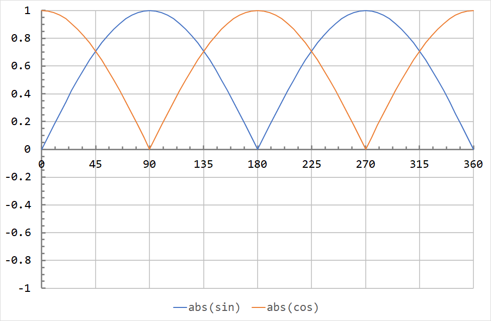
The exact mathematics are beyond the scope of this course, but the average of a sinusoid is \( \frac{2}{\pi} = 0.6366 \) times its peak value. If the y-axis represented volts, and a DC voltmeter were connected to the waveform above, it would read about 0.6366 V.
The average is also important because many cheaper multimeters are not "True RMS". Rather than calculating the RMS in real time like above, they measure the average waveform by rectifying and filtering, then by a constant to turn it into an RMS value.
\( U_{\mathrm{ac}} = \frac{U_{\mathrm{ac}}}{U_{\mathrm{pk}}} \cdot \frac{U_{\mathrm{pk}}}{U_{\mathrm{avg}}}\cdot U_{\mathrm{avg}} = \frac{1}{\sqrt{2}} \cdot \frac{\pi}{2} \cdot U_{\mathrm{avg}} = \frac{\pi}{2 \sqrt{2}} U_{\mathrm{avg}} \approx 1.111 U_{\mathrm{avg}} \)
This approximation works only if the waveform being measured is close to sinusoidal. In practice, voltages (except from devices like light dimmers) are mostly close to being sinusoidal. Currents in AC circuits tend not to be as sinusoidal due to transformers and electronic loads.